2 Preliminaries: Getting Started with RStudio

In this preliminary section, we’ll cover basic information that will help you to get started with RStudio.

2.1 R and RStudio Installation

If you haven’t already, please go ahead and install both the R and RStudio applications. R and RStudio must be installed separately; you should install R first, and then RStudio. The R application is a bare-bones computing environment that supports statistical computing using the R programming language; RStudio is a visually appealing, feature-rich, and user-friendly interface that allows users to interact with this environment in an intuitive way. Once you have both applications installed, you don’t need to open up R and RStudio separately; you only need to open and interact with RStudio (which will run R in the background).

The following subsections provide instructions on installing R and RStudio for the macOS and Windows operating systems. These instructions are taken from the “Setup” section of the Data Carpentry Course entitled R for Social Scientists. The Data Carpentry page also contains installation instructions for the Linux operating system; if you’re a Linux user, please refer to that page for instructions.

The Appendix to Garret Grolemund’s book Hands on Programming with R also provides an excellent overview of the R and RStudio installation process.

2.1.1 Windows Installation Instructions

Download R from the CRAN website
Run the .exe file that was just downloaded.
Go to the RStudio download page and under Installers select the “Windows” option.
Double click the file to install RStudio
Open RStudio to make sure it works.

2.1.2 macOS Installation Instructions

Download R from the CRAN website
Select the .pkg file for the latest R version.
Double click on the downloaded file to install R.
It is also a good idea to install XQuartz, which some packages require.
Go to the RStudio download page, and under Installers select the “macOS” option.
Double click the file to install RStudio
Open RStudio to make sure it works.

2.2 The RStudio Interface

Now that we’ve installed and opened up RStudio, let’s familiarize ourselves with the RStudio interface. When we open up RStudio, we’ll see a window that looks something like this:

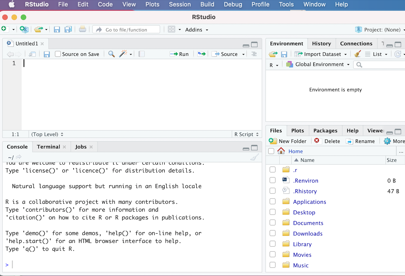
Figure 2.1: The RStudio Interface

If your interface doesn’t look exactly like this, it shouldn’t be a problem; we would expect to see minor cosmetic differences in the appearance of the interface across operating systems and computers (based on how they’re configured). However, you should see four distinct windows within the larger RStudio interface:

The top-left window is known as the Source window.
- The Source window is where we can write our R scripts (including the code associated with this tutorial), and execute those scripts. We can also type in R code into the “Console” window (bottom-left window), but it is preferable to write our code in a script within the source window. That’s because scripts can be saved (while code written into the console cannot); writing scripts therefore allows us to keep track of what we’re doing, and facilitates the reproducibility of our work. Note that in some cases, we may not see a Source window when we first open RStudio. In that case, to start a new script, simply click the File button on the RStudio menu bar, scroll down to New File button, and then select R Script from the menu bar that opens up.
- It’s also worth noting that the outputs of certain functions will appear in the Source window. In the context of our tutorial, when we want to view our datasets, we will use the View() function, which will display the relevant data within a new tab in the Source window.
The top-right window is the Environment/History pane of the RStudio interface.
- The “Environment” tab of this window provides information on the datasets we’ve loaded into RStudio, as well as objects we have defined (we’ll talk about objects more later in the tutorial). -The “History” tab of the window provides a record of the R commands we’ve run in a given session.
The bottom-right window is the Files/Plots/Packages/Help/Viewer window.
- The “Files” tab displays our computer’s directories and file structures and allows us to navigate through them without having to leave the R environment.
- The “Plots” tab is the tab where we can view any visualizations that we create. Within the “Plots” tab, make note of the “Zoom” button, which we can use to enlarge the display of our visualizations if they’re too compressed in the “Plots” window. Also, note the “Export” button within the “Plots” tab (next to the “Zoom” button); we can use this button to export the displayed visualization to a .png or .jpeg file that can be used outside of RStudio.
- The “Packages” tab provides information on which packages have been installed, as well as which packages are currently loaded (more on packages in Sections 2.3 and 2.4 below)
- The “Help” tab displays documentation for R packages and functions. If you want to know more about how a package or function work, we can simply type a “?” followed by the package or function’s name (no space between the question mark and the name) and relevant information will be displayed within the “Help” tab.
- The “Viewer” tab displays HTML output. If we write code that generates an HTML file, we can view it within the “Viewer” tab.
The bottom-left window is the Console/Terminal/Jobs window.
- The “Console” tab is where we can see our code execute when we run our scripts, as well as certain outputs produced by those scripts. In addition, if there are any error or warning messages, they will be printed to the “Console” tab. We can also type code directly into the console, but as we noted earlier, it is better practice to write our code in a script and then run it from there.
- The “Terminal”, “R Markdown” and “Jobs” tabs are not relevant for our workshop.

2.3 Install Packages

R is an open-source programming language for statistical computing that allows users to carry out a wide range of data analysis and visualization tasks (among other things). One of the big advantages of using R is that it has a very large user community among social scientists, statisticians, and digital humanists, who frequently publish R packages. One might think of packages as workbooks of sorts, which contain a well-integrated set of R functions, scripts, data, and documentation; these “workbooks” are designed to facilitate certain tasks or implement useful procedures. These packages are then shared with the broader R user community, and at this point, anyone who needs to accomplish the tasks to which the package addresses itself can use the package in the context of their own projects. The ability to use published packages considerably simplifies the work of digital humanists using R; it means that they rarely have to write code entirely from scratch, and can build on the code that others have published in the form of packages. This allows applied researchers to focus on substantive problems, without having to get too bogged down in complicated programming tasks.

In the context of this tutorial, extracting even basic information from a text corpus in R would be a relatively complex task if we had to write all our code from scratch. However, because we are able to make use of text mining and visualization packages written by other researchers and programmers, the task is considerably simpler, and will not require any complicated programming.

In this workshop, we will use the following packages to carry out some basic text mining and data visualization tasks (please click the relevant link to learn more about a given package; note that the tidyverse is not a single package, but rather an entire suite of packages used for common data science and analysis tasks):

To install a package in R, we can use the install.packages() function. A function is essentially a programming construct that takes a specified input, runs this input (called an “argument”) through a set of procedures, and returns an output. In the code block below, the name of the package we want to install (here, “tm”) is enclosed within quotation marks and placed within parentheses after printing install.packages Running the code below will effectively download the tm package to our computer:

# Installs "tm" package
install.packages("tm")

To run this code in your own R session:

First, copy the code from the codeblock above (you can copy the code to your clipboard by hovering over the top-right of the code-block and clicking the “copy” icon; you can also highlight the code and copy from the Edit menu of your browser).
Then, start a new R script within RStudio; if you want to keep a future record of your work, you may want to save this script to your computer (perhaps in the same folder to which you downloaded the tutorial data). We can save our scripts via the RStudio “File” menu.
Paste the code into the script, highlight it, and click the “Run” button that is just above the Source window.
Alternatively, instead of copying/pasting, you can manually type in the code from the codeblock into your script (manually typing in the code is slower, but often a better way to learn than copy/pasting).
After you’ve run the code, watch the code execute in the console, and look for a message confirming that the package has been successfully installed.

Below, we can see how that line of code should look in your script, and how to run it:

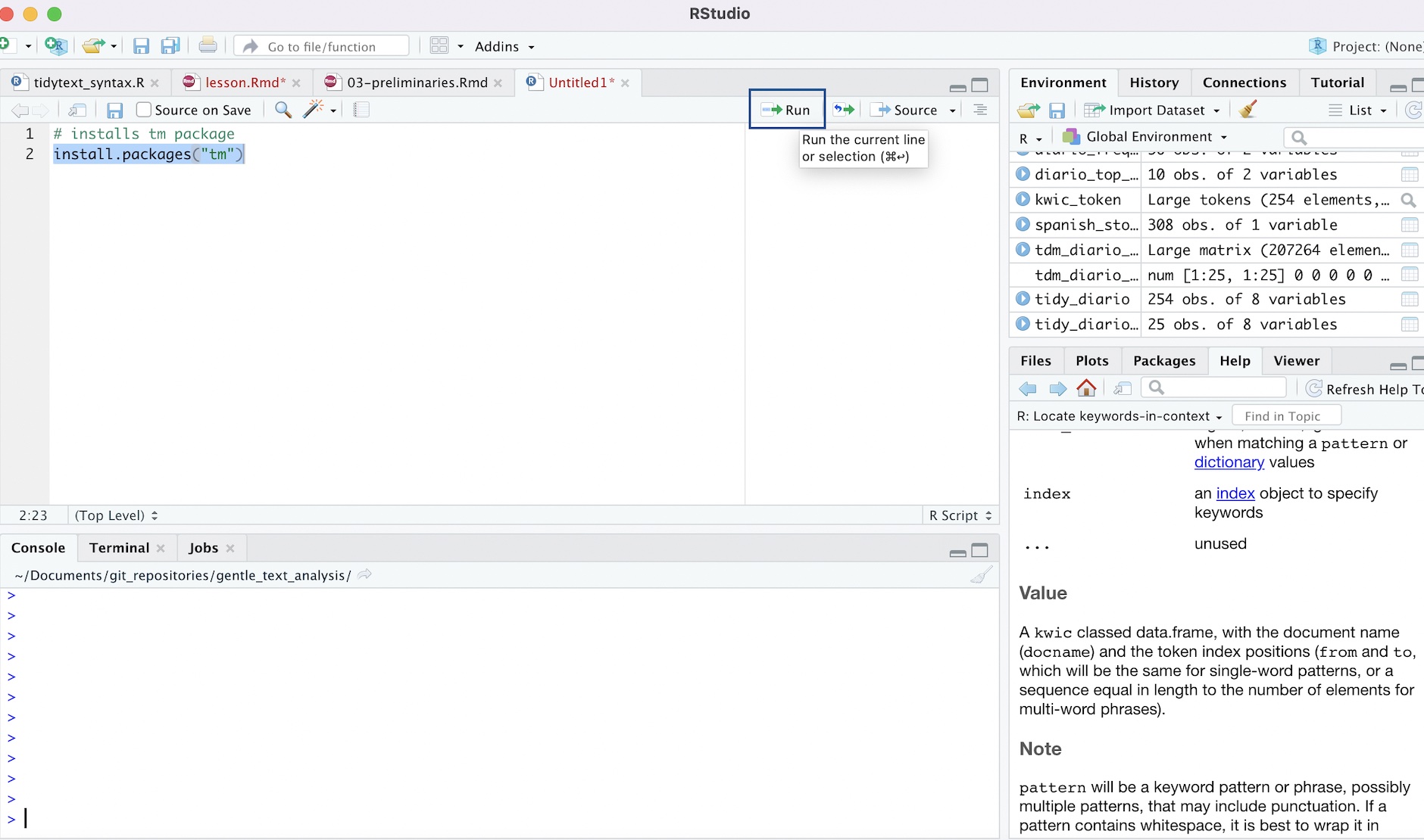
Figure 2.2: Installing tm package in R Script

Please note that you can follow along with the tutorial on your own computers by transferring all of the subsequent codeblocks into your script in just this way. Run each codeblock in your RStudio environment as you go, and you should be able to replicate the entire tutorial on your computer. You can copy-paste the workshop code if you wish, but we recommend actually retyping the code into your script, since this will help you to more effectively familiarize yourself with the process of writing code in R.

Note that the codeblocks in the tutorial usually have a comment, prefaced by a hash (“#”). When writing code in R (or any other command-line interface) it is good practice to preface one’s code with brief comments that describe what a block of code is doing. Writing these comments can allow someone else (or your future self) to read and quickly understand the code more easily than otherwise might be the case. The hash before the comment effectively tells R that the subsequent text is a comment, and should be ignored when running a script. If one does not preface the comment with a hash, R wouldn’t know to ignore the comment, and would throw an error message.

Now, let’s install the other packages we mentioned above, using the same install.packages() function:

install.packages("tidyverse")
install.packages("wordcloud2")
install.packages("quanteda")
install.packages("tidytext")

All of the packages we need are now installed!

2.4 Load libraries

However, while our packages are installed, they are not yet ready to use. Before we can use our packages, we must load them into our environment. We can think of the process of loading installed packages into a current R environment as analogous to opening up an application on your phone or computer after it has been installed (even after an application has been installed, you can’t use it until you open it!). To load (i.e. “open”) an R package, we pass the name of the package we want to load as an argument to the library() function. For example, if we want to load the tm package into the current environment, we can type:

# Loads tm package into memory
library(tm)

At this point, the full suite of the tm package’s functionality is available for us to use.

Now, let’s go ahead and load the remainder of the packages that we’ll need:

# loads remainder of required packages
library(tidyverse)
library(wordcloud2)
library(quanteda)
library(tidytext)

At this point, the packages are loaded and ready to go! One important thing to note regarding the installation and loading of packages is that we only have to install packages once; after a package is installed, there is no need to subsequently reinstall it. However, we must load the packages we need (using the library function) every time we open a new R session. In other words, if we were to close RStudio at this point and open it up later, we would not need to install these packages again, but would need to load the packages again.

2.5 Set working directory

Before we can bring our workshop data into RStudio and begin the tutorial, we have to specify that data’s location on our computer. This step is known as setting one’s working directory. First, make sure that you’ve downloaded the Diario text data, and have placed it in a directory (i.e. folder) on your computer that is specifically dedicated to this tutorial. To complete the workshop tasks, you will want to set your working directory to the “creatives” subdirectory within the main “2019.11.14-ElDiarioCorpus” directory that you downloaded.

If you’re unfamiliar with the concept of file paths, the easiest way to set your working directory is through the RStudio menu. To use this option, follow these steps:

First, Click on the “Session” menu on the RStudio menu bar at the top of your screen, and then scroll down to the “Set Working Directory” button in the menu that opens up.
When you hover over the “Set Working Directory” button, a subsidiary menu that contains a button that says “Choose Directory” will open; click this “Choose Directory” button.
In the dialog box that opens up, navigate to the “creatives” subdirectory within the “2019.11.14-ElDiarioCorpus” folder, select it, and click “Open”. At this point, your working directory should be set!

The graphic below demonstrates the process of setting one’s working directory through RStudio’s menus:

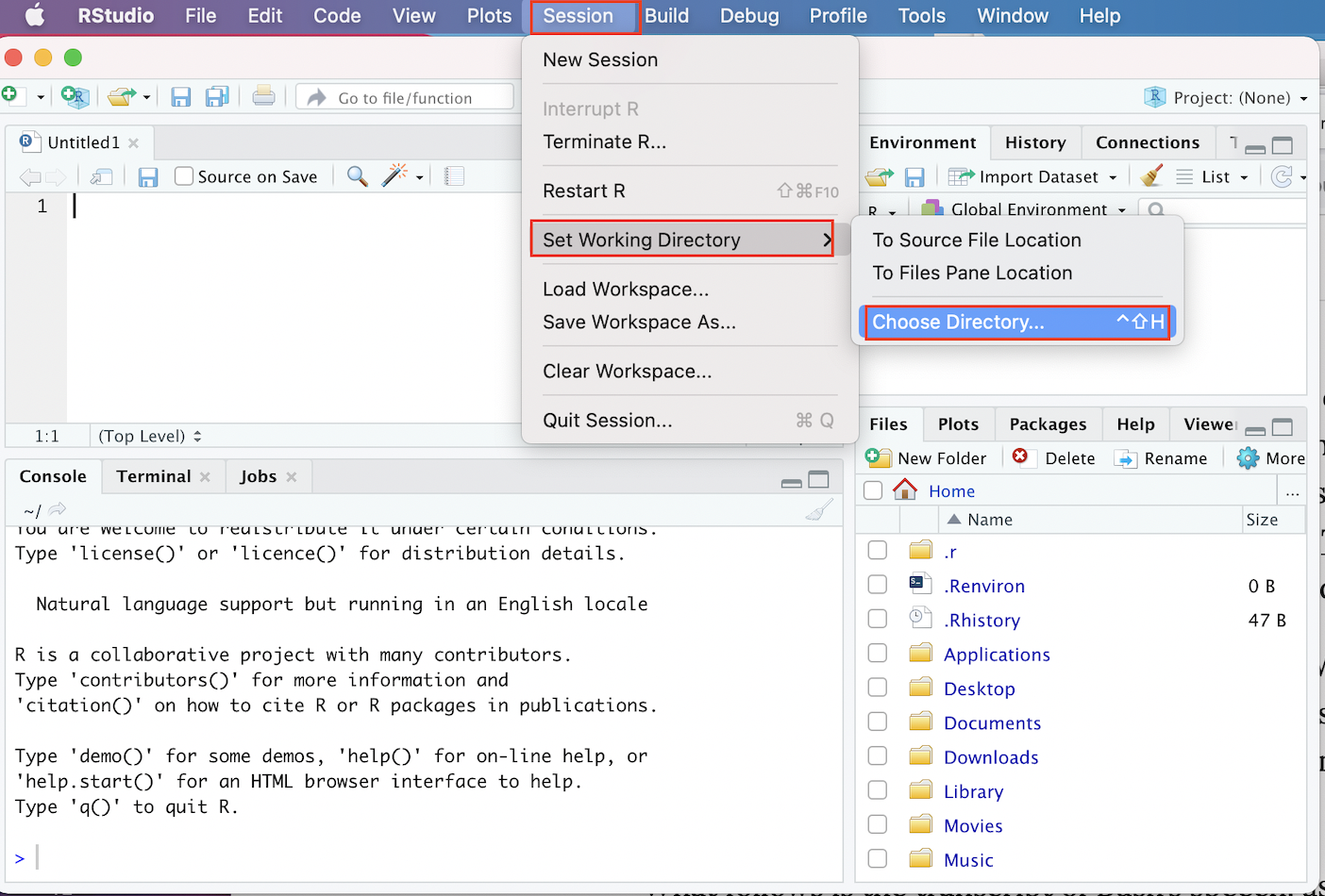
Figure 2.3: Setting Working Directory Via Menus

Alternatively, if you are familiar with the concept of file paths, and know the file path to the folder containing the downloaded El Diario “creatives” text files, you can directly set the working directory using the setwd() function, where the argument to the function is the relevant file path enclosed in quotation marks. For example, the following code sets the working directory to the folder containing the creatives from the El Diario corpus:

# Sets working directory 
setwd("019.11.14-ElDiarioCorpus/creatives")

Note that you won’t want to copy and paste the above codeblock, since your file path may be different; be sure to replace the file path above with your own.