7 Refining and formatting maps

In the previous section, we created and refined two maps based on the index of racial bias in traffic stops we created earlier in the tutorial. The first map shows the spatial distribution of the continuous “bias_index” variable across counties.

It looked like this:

# prints "traffic_bias_map_continuous"
traffic_bias_map_continuous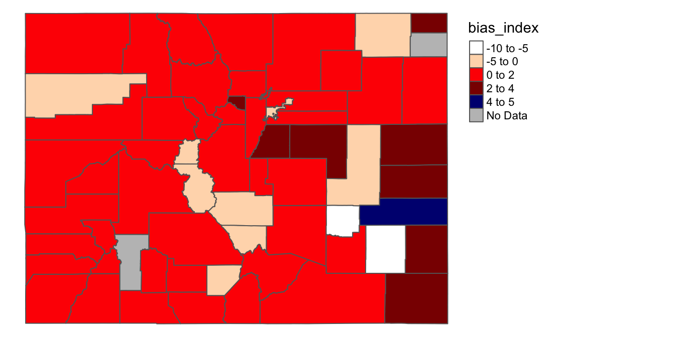

The second map created a new categorical variable based on “bias_index”, and displayed these categories on a map.

It looked like this:

# prints "traffic_bias_map_categorical"
traffic_bias_map_categorical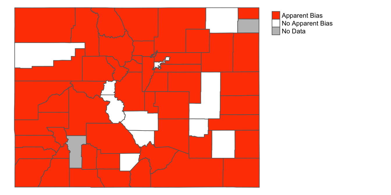

In this section, we’ll continue to refine and customize these maps (for example, by adding titles, map credits, county labels, and labels and titles for the legend).

7.1 Refine the map of the continuous “bias_index” variable

Let’s start by fine-tuning the map of the continuous “bias_index” variable. As an exercise, read through the code below (without scrolling down to the map), and see if you can decipher what each line is doing, forming a mental picture of the in-progress map as you go. If you’re having trouble understanding something, look up the function’s documentation, which yoi can access by typing the name of the function, preceded by a question mark. For example, if we want to access the documentation for the tm_polygons() function, we can type ?tm_polygons, which will bring up the function’s documentation (which provides a description of the various arguments to the function), in the “Help” tab on the bottom-right of the R Studio interface.

my_colors<-c("white", "peachpuff", "red1", "red4", "navy")

traffic_bias_map_continuous<-
tm_shape(county_shapefile_biasIndex)+
  tm_polygons(col="bias_index", 
              palette=my_colors,
              title="(Black % of Traffic Stops) - (Black % of Population)",
              textNA="No Data", 
              breaks=c(-10,-5, 0.01, 2, 4, 5))+
  tm_layout(frame=FALSE, 
            legend.outside=TRUE,
            legend.text.size=0.68,
            legend.title.size=0.75,
            title.size=0.75,
            title.fontface = 2,
            title="Traffic Stop Racial Bias Index",
            main.title="Racial Bias in Traffic Stops, by County (Colorado)",
            main.title.position=0.03,
            main.title.size=1,
            attr.outside=TRUE)+
  tm_credits("Map Author: NAME\nData Sources: 2010 Decennial Census via tidycensus,\nStanford Open Policing Project,\nColorado GeoLibrary ", 
            position=c(0.02,0.01),
            size=0.38)

Having read through this code, let’s see what that the resulting map looks like:

# prints updated map assigned to "traffic_stop_map_continuous" object
traffic_bias_map_continuous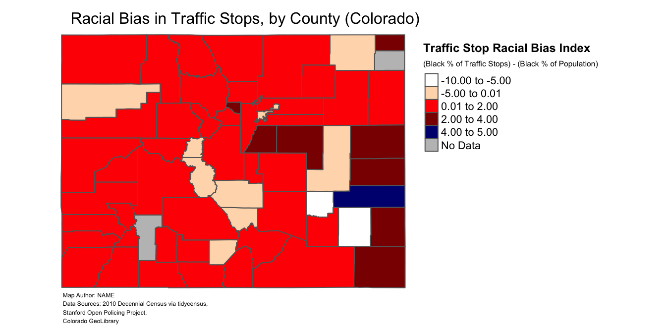

Now, let’s unpack the various components of the code.

The code begins by defining the my_colors vector; this is the same color vector we used in Section 6.3.3, and is reproduced for convenience here.
traffic_bias_map_continuous<- indicates that the map created through the code on the right side of the assignment operator will be assigned to the object named traffic_bias_map_continuous. This overwrites the previous version of the map assigned to this object.
The first function that is called is tm_shape(); we pass the name of the object that contains the data we want to map to this function, which yields tm_shape(county_shapefile_biasIndex).
After specifying our dataset with tm_shape(), we call the tm_polygons() function. The tm_polygons() function takes several arguments, beginning with col="bias_index (which specifies the column within county_shapefile_biasIndex that we want to map), and palette=my_colors (which specifies that we want to use the colors from the my_colors vector to represent different interval ranges for the “bias_index” variable). Next, in title="(Black % of Traffic Stops) - (Black % of Population), we define a subtitle for the legend, so that viewers of the map can discern the intuition behind the bias index that is being mapped. Finally, textNA="No Data" defines the legend label for “NA” values, and breaks=c(-10,-5, 0.01, 2, 4, 5) sets the data intervals, which are communicated in the map’s legend. Notice that instead of setting one of the break points at 0, this version of the map uses 0.01; that is because the lower bound on data intervals is inclusive, while the upper bound is exclusive (i.e. a hypothetical county with a bias index of exactly 4.00 would be assigned the color that corresponds with the 4.00 to 5.00 legend interval, not the one corresponding to 2.00 to 4.00). As a result, a county with a bias index value of exactly zero would be grouped with counties with a positive value on the index, when it would make more sense to group such a county with counties with negative values on the index. Setting the break point slightly above 0 avoids a scenario where a county with an index value of exactly 0 is grouped together with counties with an index value greater than zero.
The next tmap function that is called is the tm_layout() function, which allows us to specify various parameters that shape the map’s layout. Recall from before that frame=FALSE removes the map’s bounding box (which surrounds the area displayed on the map), while legend.outside=TRUE places the legend outside the map’s domain, so that it doesn’t overlap with any of the counties that are displayed. Next, legend.text.size=0.68 sets the size for legend text elements (that are not part of the legend’s title or subtitle), while legend.title.size=0.75 sets the size of the legend’s subtitle, and title.size=0.75 sets the size of the text in the legend’s main title. Note that when setting the size of text elements on your map, the best approach to use is usually trial and error; start with an arbitrary size, and then iterate from there. title="Traffic Stop Racial Bias Index" sets the text for legend’s main title, and title.fontface = 2 sets the legend’s main title text in boldface. main.title="Racial Bias in Traffic Stops, by County (Colorado)" sets the map’s main title, main.title.position=0.03 sets the position/justification of the title, and main.title.size=1 sets the size of the main title’s text. Finally, attr.outside=TRUE specifies that any map elements other than the legend (such as the map credits) are to be placed outside the map boundary.
The tm_credits() function is a tmap function which allows us to add a credits section to the map, to convey information about things such as the name of the map author and the sources of the data used to create the map. In the code above, the first argument to the tm_credits() function is simply the text we would like to include in the credits; new lines are indicated by text that reads \n. Second, position=c(0.02,0.01) specifies the position of the credits section with respect to the map (the first element of the vector, 0.02, can be thought of as the x-coordinate, while the second element, 0.01, can be thought of as a y-coordinate); these coordinates place the credits below the map on the left-hand side. Finally, size=0.38 specifies the size of the text used in the credits section.

Notice that our map currently does not have labels for county names; these can easily be added using the tm_text() function that is part of the tmap package. Instead of rewriting all of the code from above, we can simply append the tm_text() function and its arguments to the map object we already created above (traffic_bias_map_continuous). The code below takes the existing traffic_bias_map_continous object, which we updated above, and adds a line of code that reads tm_text("NAME", size=0.30, fontface=2). This labels the map’s polygons using information from the underlying dataset’s “NAME” field (which contains county names), using a text size of 0.3; the argument fontface=2 specifies that the county name labels are to be printed in boldface. No other changes or additions are made to traffic_bias_map_continuous. The version of the map that is labelled is assigned to a new object, named traffic_bias_map_continuous_labeled.

# Adds labels to "traffic_bias_map_continuous" and assigns new labeled map
# to new object named "traffic_bias_map_continuous_labeled"
traffic_bias_map_continuous_labeled<-
  traffic_bias_map_continuous+
    tm_text("NAME", size=0.30, fontface=2)

When we open traffic_bias_map_continuous_labeled, we can see the map with labels:

# prints contents of "traffic_bias_map_continuous_labeled"
traffic_bias_map_continuous_labeled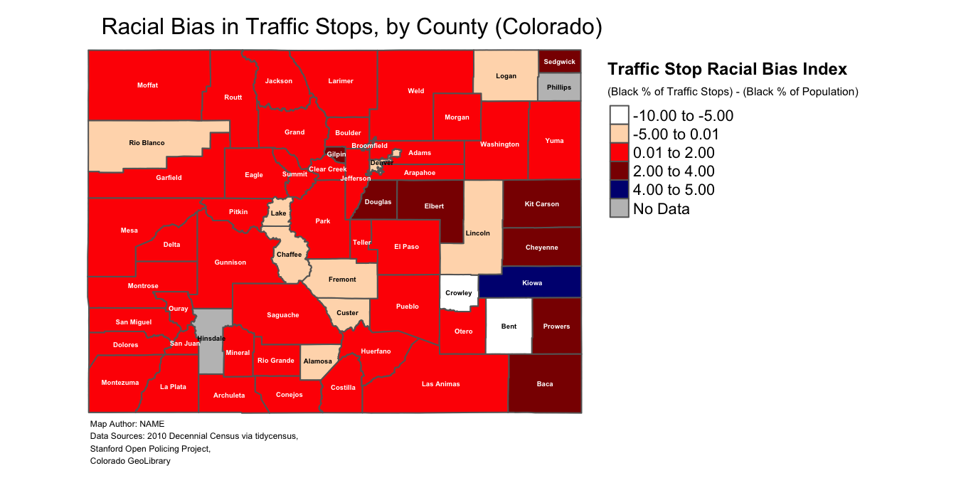

7.2 Refine the categorical map

The code below refines the categorical map we created in Section 6.4. The map is largely the same as the one created in that section, but adds and customizes the appearance of the map’s title using arguments to the tm_layout() function that we have already discussed in Section 7.1, and also adds a map credits section that is identical to the one we used in 7.1. The map is assigned to the traffic_bias_map_categorical object, which overwrites the map we previously assigned to this object in Section 6.4.

traffic_bias_map_categorical<-
tm_shape(county_shapefile_biasIndex)+
  tm_polygons(col="apparent_bias", 
              title="", 
              palette=c("orangered1", "white"), 
              textNA="No Data")+
    tm_layout(frame=FALSE, 
              legend.outside=TRUE,
              main.title="Racial Bias in Traffic Stops, by County in Colorado\n(Based on Whether % of Black Motorists Stopped by Police > County's Adult Black Population %)",
              main.title.position=0.03,
              main.title.size=0.75,
              attr.outside=TRUE)+
  tm_credits("Map Author: NAME\nData Sources: 2010 Decennial Census via tidycensus,\nStanford Open Policing Project,\nColorado GeoLibrary ",
              position=c(0.02,0.01), # Specifies location of map credits
             size=0.38)+
  tm_text("NAME", size=0.30, fontface=2)

We can print the contents of traffic_bias_map_categorical to view the updated map in the “Plots” window:

# prints contents of "traffic_bias_map_categorical"
traffic_bias_map_categorical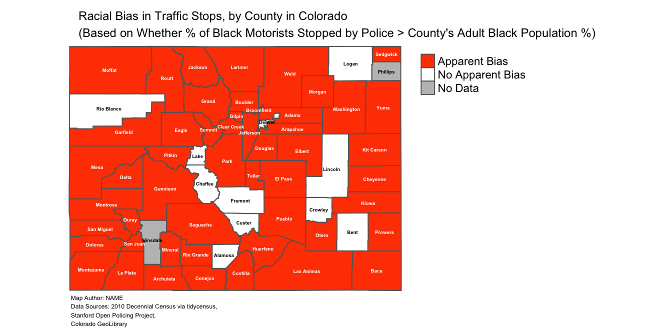

7.3 Create a dynamic map of the bias index

Recall from Section 6.1 that it is possible to render both static maps and interactive maps using the tmap package. Thus far, our focus has been on creating static maps to display county-level variation in the “bias_index” variable (or the derivative “apparent_bias” variable). It’s worth briefly reminding ourselves that we can easily turn these static maps into dynamic maps by changing the tmap mode to “view.” For example, let’s say we want to display the map assigned to traffic_bias_map_continuous in a dynamic setting:

# Changes tmap mode to "view"
tmap_mode("view")

## tmap mode set to interactive viewing

# Prints "traffic_bias_map_continuous" in View mode
traffic_bias_map_continuous

## Credits not supported in view mode.