Shiny Fundamentals
Last updated on 2025-12-30 | Edit this page
Overview
Questions
- What are the different components of a Shiny application and how do they fit together?
- How can we create, run, and view a simple Shiny application?
- How can we create an interactive Shiny application that is responsive to user inputs or requests?
- How can we customize the appearance of a simple Shiny application?
Objectives
- Explain how to use markdown with the new lesson template
- Demonstrate how to include pieces of code, figures, and nested challenge blocks
Preliminaries
Before beginning this episode, please load the following libraries”
R
# load libraries
library(shiny)
library(shinythemes)
library(shinyjs)
OUTPUT
Attaching package: 'shinyjs'OUTPUT
The following object is masked from 'package:shiny':

    runExample
OUTPUT
The following objects are masked from 'package:methods':

    removeClass, show
The Structure of a Shiny Application
At the conclusion of the previous Episode, we examined some currently published Shiny applications. Now, we’ll begin peeking “under the hood” to see how these applications are put together, and how they work. Our starting point is the observation that all Shiny applications, no matter how complex, have three fundamental and interrelated building blocks:
- A user interface (UI) that specifies the appearance and layout of the application
- A server that defines how an application generates outputs in response to user inputs
- A call to the
shinyApp()function, which launches the application by bringing together the UI and server
The relationship between the user interface and server is dynamic and bi-directional; the server provides substantive content (created using R code) that populates the user interface, while the user interface defines how that content is organized and displayed to users. This may sound fairly abstract, but will hopefully come into focus as we proceed.
Our first application: Hello, World!
In this section, we’ll develop our very first Shiny application. There’s a good chance that the first (or one of the first) things you did in R was to print a “Hello, World” statement:
R
# prints "Hello, World"
print("Hello, World")
OUTPUT
[1] "Hello, World"Our goal in this section is to wrap this statement into a “Hello, World” Shiny application.
A note on application files and directories
First, though, it is important to briefly discuss where to write and store your applications. Ideally, you should create a separate dedicated directory for each application you write. For now, we’ll create our application scripts, containing the UI and server code, in a familiar .R file (but R Studio does have a handy pre-built template for Shiny applications, which we’ll introduce later on). This application directory can also contain other elements relevant to or referenced by your application (such as image files, datasets, Readme files etc.). As applications grow in complexity, it could make sense for you to use subdirectories to organize your main application directory.
Each R script should only contain the code for a single application; trying to include the code for multiple applications in a single script can cause errors or undefined behavior when you try to launch an application (since Shiny may be confused about which application it’s supposed to run). That said, in this episode, we’ll be creating and running several simple “toy” applications to illustrate important Shiny features. You can either save each application in separate scripts, or write all of the applications in a single script while commenting out the code for the application(s) you are NOT running; that way, you can write code for several simple applications in one .R file, while ensuring that only one script at a time is “live” when you try to launch it.
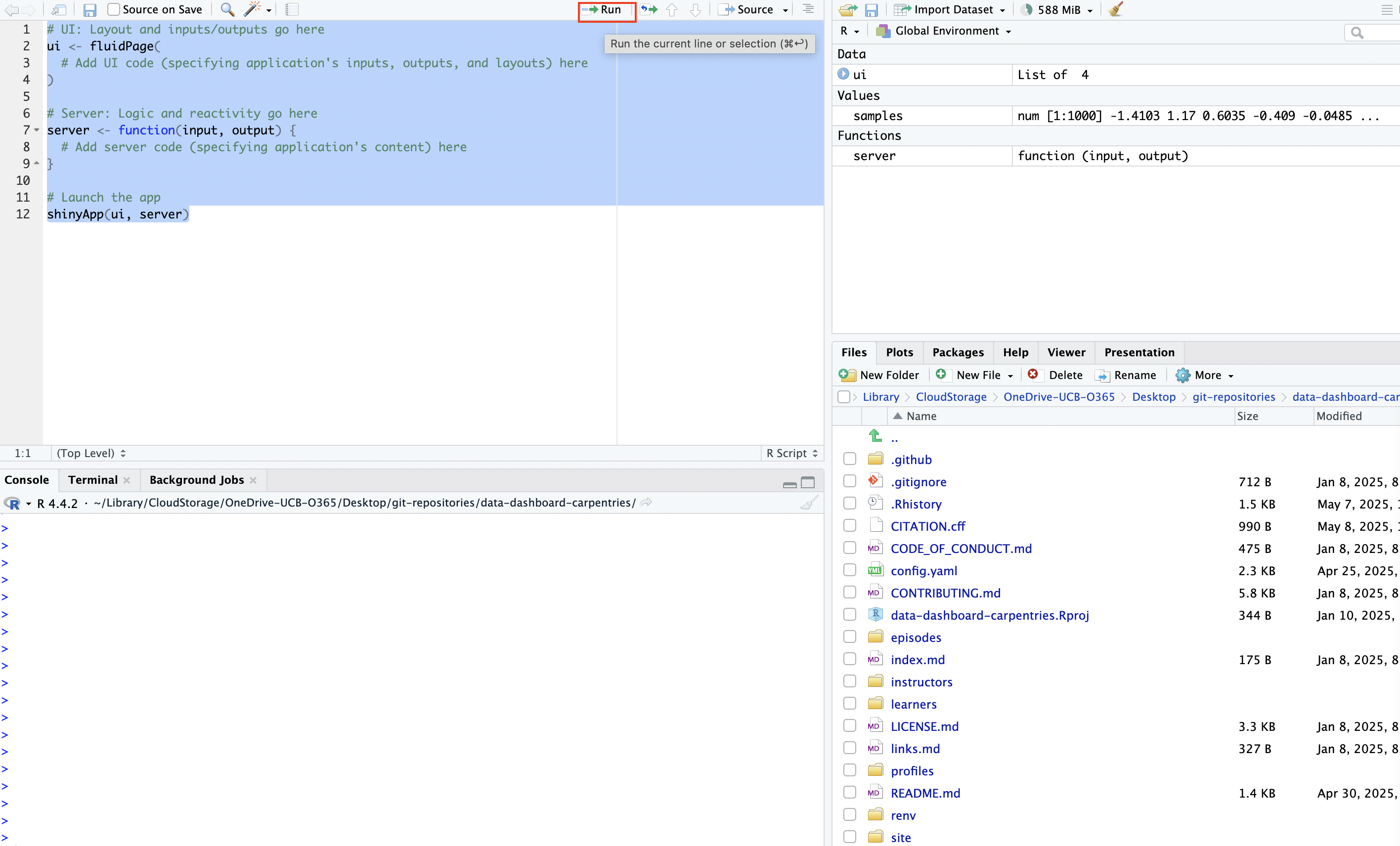
Writing the “Hello, World” application
Let’s first write out our application’s skeletal structure,
translating the three components we discussed above (the UI, server, and
shinyApp()) into actual Shiny code. After getting this
structure down, we’ll fill in elements to create the “Hello, World”
application below. Recall from above that the application’s UI defines
how the application looks (i.e. what are the inputs and
outputs, and how are they visually displayed), the server defines what
the application does and how it works (i.e. how inputs are
processed to generate outputs), and the call to shinyApp()
brings these elements together to launch the application.
R
# UI: Layout and inputs/outputs go here
ui <- fluidPage(
  # Add UI code (specifying application's inputs, outputs, and layouts) here
)

# Server: Logic and reactivity go here
server <- function(input, output) {
  # Add server code (specifying application's content) here
}

# Launch the app
shinyApp(ui, server)
Some aspects of this code require additional clarification.
- The
fluidPage()function used in the creation of the UI object is a Shiny layout function that creates a responsive web page layout that automatically adjusts to different screen sizes. The arguments tofluidPage(), will contain additional functions that define the user interface. - Within the server function, “input” is used to access values the user has entered or selected in the UI, while “output” is used to define the content that is displayed within the UI. Sometimes, in more complex applications with more sophisticated user interfaces, you will also see a “session” argument in the server function, but that is beyond the scope of our current workshop.
Again, this may still seem a little but abstract, but will hopefully
come into focus as we proceed. You can launch an application from your
script by simply running the UI and server code, along with with
shinyApp(ui, server):
Since our application is still empty, launching it will generate a blank page that looks something like this:

Now, let’s go ahead and create our “Hello, World” app by adding this text to the application structure we’ve defined above. It may not seem intuitive at first, but we’ll unpack it after writing out the code and launching the application.
R
# UI: Layout and inputs/outputs go here
ui <- fluidPage(
  textOutput(outputId="greeting")  # Placeholder for text
)

# Server: Logic and reactivity go here
server <- function(input, output) {
  # Add server code (specifying application's text)
  output$greeting <- renderText({
    "Hello, World!"  # application content
  })
}

# Launch the app
shinyApp(ui, server)
When you go ahead and launch this application from your .R file, you’ll see something that looks like this:
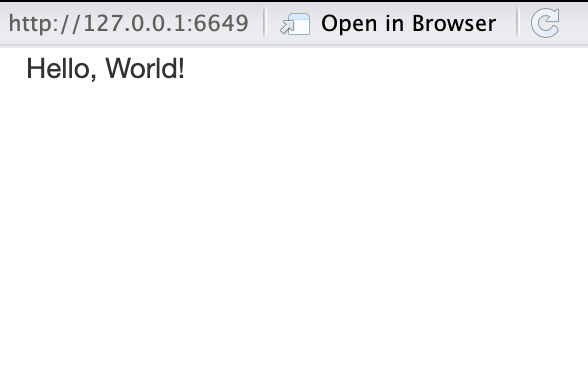
Congratulations on writing your first Shiny application!
This application was simple–it’s just a blank web page with “Hello,
World!” written on it–but it’s certainly less intuitive than printing
that string to the console with Hello, World. The code
above needs some unpacking:
-
textOutput()is one of Shiny’s UI output functions; it creates a placeholder in the user interface for a text string that will be defined in the server. The argument to this function, “greeting”, is an arbitrary identifier that will be used to link the text string defined in the server back to this placeholder in the user interface. To learn more abouttextOutput()please consult the documentation with?textOutput(). - After creating the placeholder for text output in the UI, the server
defines what text will be displayed in the UI with
output$greeting <- renderText({"Hello, World!"}).renderText()is a server-side output function used to generate the text displayed in the placeholder created bytextOutput(). In Shiny,output()is a special object that is used to store content that will be displayed in the UI. Shiny uses dollar sign notation to assign the content in the output object to a specific UI placeholder, identified by its output ID. Here,output$greetingconnects the rendered text to the UI placeholder identified byoutputId="greeting".
In Shiny, output functions determine what gets displayed in the application. These are used to show text, plots, tables, or other content, either by reserving space in the UI (UI output functions) or by generating content in the server (server-side output functions).
Output functions in the UI are sometimes referred to as “placeholder functions” because they reserve space in the UI where content created in the server will appear.
Output functions in the server are sometimes referred to as “render functions”, because they generate (or “render”) the content that fills the placeholders defined in the UI.
Each render function in the server has a matching placeholder in the
UI. For example, in the simple “Hello, World!” app, the placeholder
function textOutput() reserves space in the UI, while the
corresponding render function renderText() generates the
text that will be shown there.
Shiny connects the two using output$id where “id”
matches the identifier given to the placeholder.The content returned by
the render function is displayed in the UI at the location specified by
the placeholder.
Challenge 1: Make your own text app
Using what you’ve learned above, make your own basic Shiny application that communicates a message in simple text. Rather than simply modifying the “Hello, World!” app, write it from scratch; this will help you become familiar with Shiny’s syntax.
Displaying a plot in a Shiny application
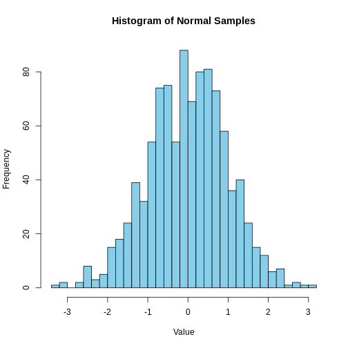
Instead of printing a text string in our application, let’s instead
create a Shiny application that displays a simple plot that’s generated
with some R code. Below, we generate 1000 random values from a normal
distribution with a mean of 0 and a standard deviation of 1, and assign
the resulting vector to a new object named samples. We then
plot a histogram of the samples data that’s divided into 30
bins:
R
# create a vector of 1000 randomly generated values from a normal distribution with a mean of 0 and SD of 1
samples <- rnorm(1000, mean = 0, sd = 1)

# make a histogram of "samples" data
hist(samples, breaks = 30, col = "skyblue",
     main = "Histogram of Normal Samples",
     xlab = "Value")
Let’s wrap this histogram into a simple Shiny app; we’ll do so in much the same way we wrapped “Hello, World” into a Shiny app, with some minor adjustments to account for the fact that we want to display a plot, rather than text. In particular, we’ll use a new set of output functions designed specifically for plots (rather than output functions designed for text, as above). Let’s start by first creating the skeletal structure for a blank application:
R
# UI: Layout and inputs/outputs go here
ui <- fluidPage(
  # Add UI code (specifying application's inputs, outputs, and layouts) here
)

# Server: Logic and reactivity go here
server <- function(input, output) {
  # Add server code (specifying application's content) here
}

# Launch the app
shinyApp(ui, server)
Now, let’s begin populating the application:
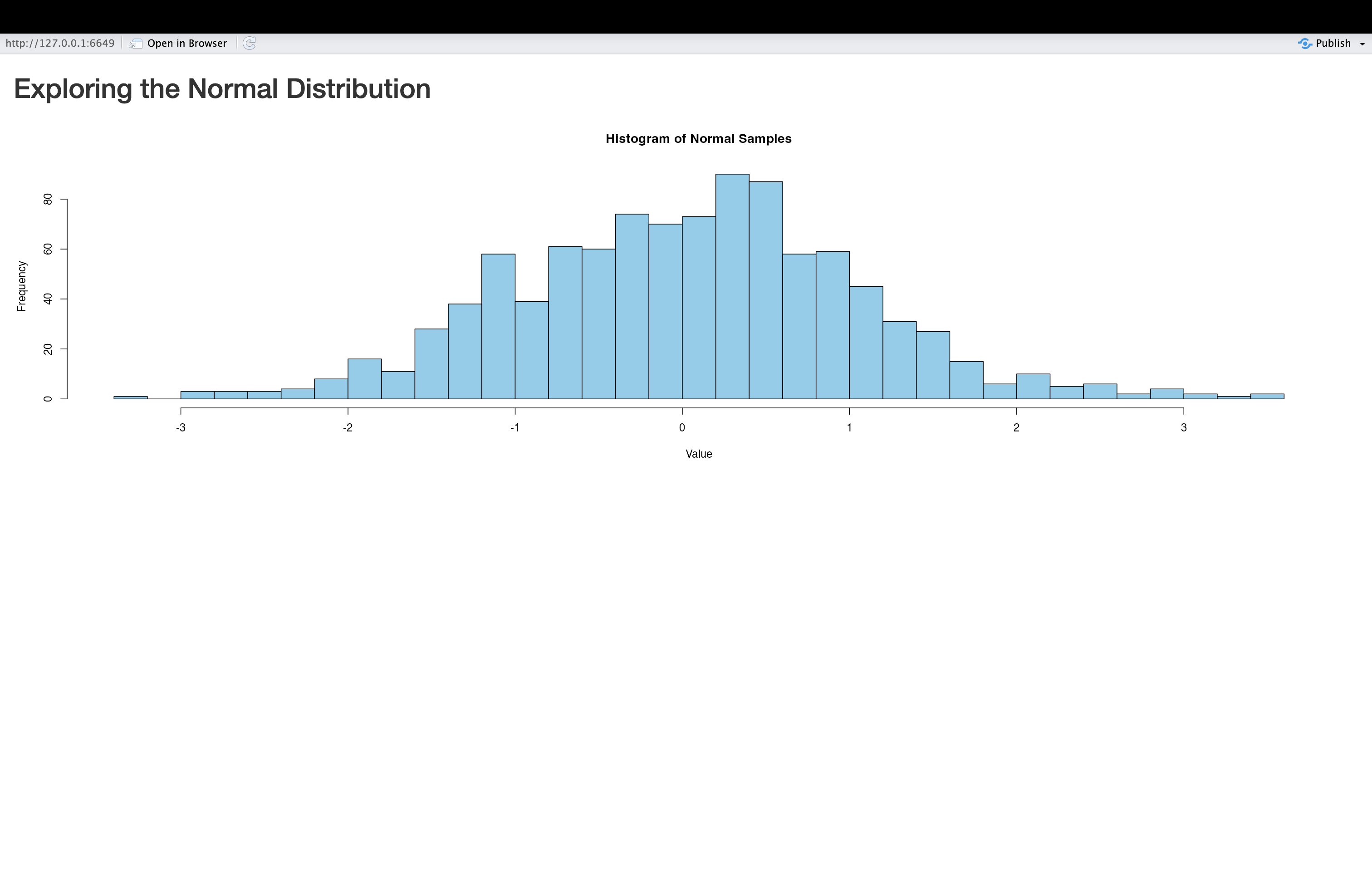
- In the “Hello, World!” application, we didn’t make a title for the
application. That can be a useful thing to do, so here, we’ll create a
title for the application using Shiny’s
titlePanel()function. We’ll name the application “Exploring the Normal Distribution”, which we can pass as an argument totitlePanel()in the UI. - We’ll create a placeholder for the plot in the UI using Shiny’s
plotOutput()function, and use “normal_plot” as the output ID. Note that different elements in the UI are separated by a comma (in this case, a comma separates thetitlePanel()andplotOutput()functions) - Then, in the server, we’ll wrap the code to make our plot within the
renderPlot()function, and assign this output back to the UI using the “normal_plot” ID.
Our application code should look something like this:
R
# UI: Layout and inputs/outputs go here
ui <- fluidPage(
  # Add UI code (specifying application's inputs, outputs, and layouts) here
  titlePanel("Exploring the Normal Distribution"),
  plotOutput(outputId = "normal_plot")
)

# Server: Logic and reactivity go here
server <- function(input, output) {
  # Add server code (specifying application's content) here
  output$normal_plot<-renderPlot({
    # create vector
    samples <- rnorm(1000, mean = 0, sd = 1)

    # make a histogram of "samples" data
    hist(samples, breaks = 30, col = "skyblue",
         main = "Histogram of Normal Samples",
         xlab = "Value")
  })
}

# Launch the app
shinyApp(ui, server)
When you’re ready, go ahead and launch the application. It will look something like this:
Applications with multiple outputs
The “Hello, World!” application displayed a text output, while the
app we just created displayed a plot output. There’s no reason why a
Shiny application cannot include many different types of outputs
(indeed, most “real world” Shiny apps do!). Let’s now make a slightly
more complex application that incorporates both text and plot outputs;
we’ll use the same plot as above, and add some text to provide some
additional context, using textOutput() to create a
placeholder in the UI, and the renderText() function to
create the message we’d like to display. The output created using
renderText() is assigned back to the UI placeholder by
using dollar sign notation to reference the output ID specified in
textOutput(). Your application code should look something
like the following:
R
# UI: Layout and inputs/outputs go here
ui <- fluidPage(
  # Add UI code (specifying application's inputs, outputs, and layouts) here
  titlePanel("Exploring the Normal Distribution"),
  textOutput(outputId="context_discussion"),
  plotOutput(outputId = "normal_plot")
)

# Server: Logic and reactivity go here
server <- function(input, output) {
  # Add server code (specifying application's content) here

  # creates text output
  output$context_discussion<-renderText({
    "This histogram shows 1,000 values randomly drawn from a standard normal distribution. Most values fall between -3 and 3, with a peak around 0."
  })

  # creates plot output
  output$normal_plot<-renderPlot({
    # create vector
    samples <- rnorm(1000, mean = 0, sd = 1)

    # make a histogram of "samples" data
    hist(samples, breaks = 30, col = "skyblue",
         main = "Histogram of Normal Samples",
         xlab = "Value")
  })
}

# Launch the app
shinyApp(ui, server)
Now, let’s go ahead and launch our application, and see what it looks like:
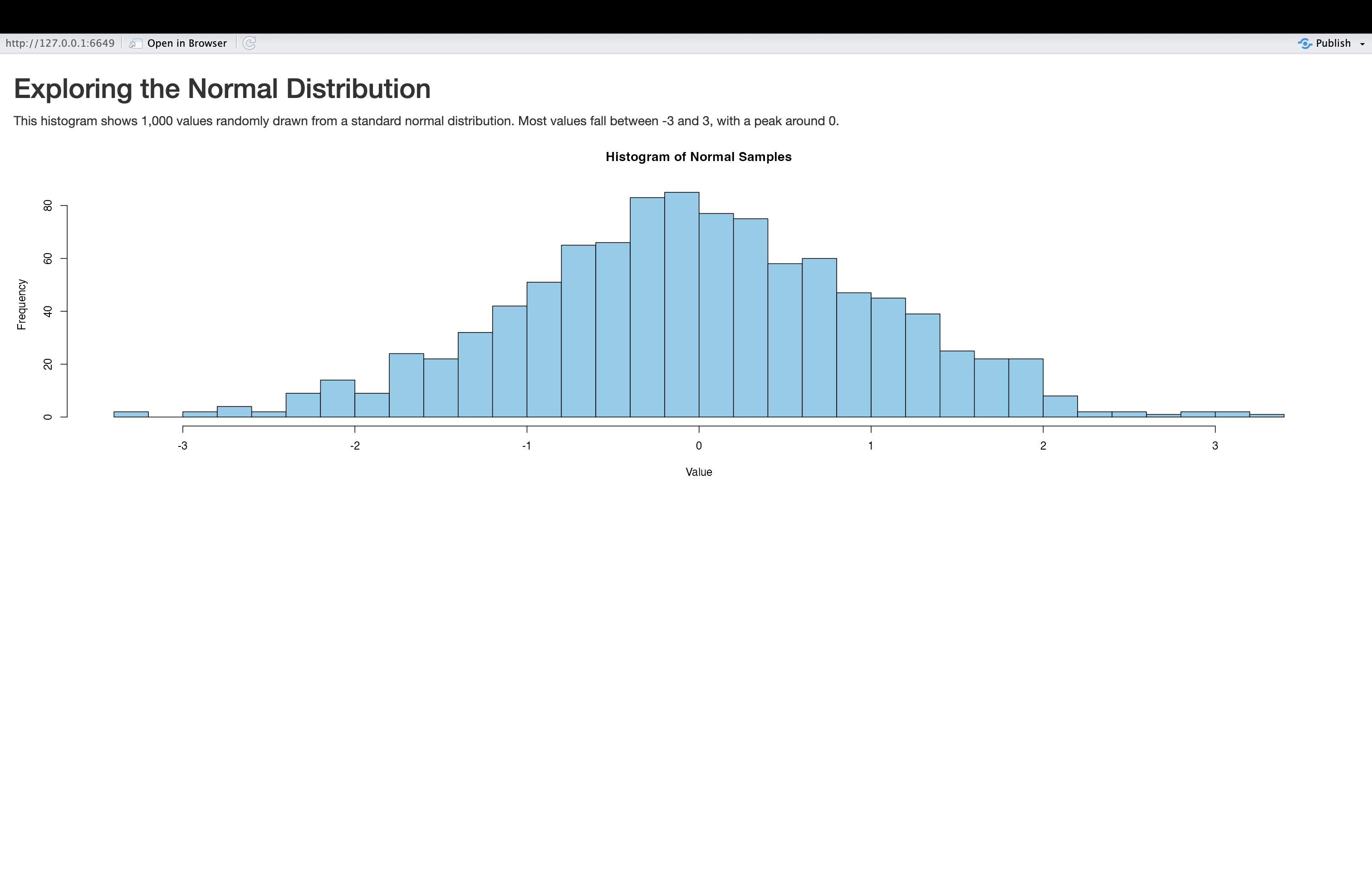
Note the text above the plot in this modified application.
Challenge 2: Change an application’s layout
In the application we just created, the written text providing relevant context is situated above the plot. Modify the application code so that it’s instead below the plot.
To make this change, you can simply move textOutput()
function below the plotOutput() function in the UI. There
is no need to change the order of anything in the server; the order in
which elements is displayed is solely governed by the UI code. The code
for a modified application with the text element below the plot looks as
follows:
R
# UI: Layout and inputs/outputs go here
ui <- fluidPage(
  # Add UI code (specifying application's inputs, outputs, and layouts) here
  titlePanel("Exploring the Normal Distribution"),
  plotOutput(outputId = "normal_plot"),
  textOutput(outputId="context_discussion")
)

# Server: Logic and reactivity go here
server <- function(input, output) {
  # Add server code (specifying application's content) here

  # creates text output
  output$context_discussion<-renderText({
    "This histogram shows 1,000 values randomly drawn from a standard normal distribution. Most values fall between -3 and 3, with a peak around 0."
  })

  # creates plot output
  output$normal_plot<-renderPlot({
    # create vector
    samples <- rnorm(1000, mean = 0, sd = 1)

    # make a histogram of "samples" data
    hist(samples, breaks = 30, col = "skyblue",
         main = "Histogram of Normal Samples",
         xlab = "Value")
  })
}

# Launch the app
shinyApp(ui, server)
A conceptual overview of interactive applications
So far, we have learned about the basic structure of Shiny applications and how to populate them with content by linking output functions in the UI (placeholder functions) with output functions in the server (render functions). You may have noticed that the applications we have built so far are static, in the sense that they don’t respond dynamically to user input. However, static applications have limited utility, and much of the power and usefulness of Shiny applications comes from their ability to dynamically respond to user input.
Input Functions
To build dynamic, interactive applications, we need to introduce a new class of Shiny functions: input functions. Input functions are UI functions that create interactive elements where users can enter or select information (such as text boxes, sliders, check boxes, or radio buttons). This user input can then determine what gets displayed in the app.
For example, imagine an app that contains some text output in the UI, and radio buttons that let the user choose a language. If the user selects “English”, the text appears in English; if they select “Spanish”, it appears in Spanish. The function that creates these radio buttons in Shiny is considered an input function.
Reactivity
In Shiny, applications respond to user input by automatically recalculating and updating outputs whenever their underlying inputs change. For example, if a user adjusts a slider input specifying a date range, any outputs depending on that slider (i.e. a plot, text, table etc.) will automatically update without needing to refresh or re-run the app. This concept is known as reactivity.
Reactivity is built into Shiny functions. For example, the
server-side renderPlot() function can explicitly reference
input values (we’ll see how to do this below); the plot will
automatically re-render whenever the user changes a relevant input
value. In other words, render functions “listen” for changes in inputs
and update their output value accordingly.
It’s worth highlighting how unique reactive behavior in Shiny is,
compared to the way the R programming language works more generally. In
particular, traditional R code is emphatically not reactive. To
make this more concrete, let’s consider an example. First, we’ll define
two new objects, x and y”
R
# defines objects x and y
x<-5
y<-x+1
As expected, we can see the value of y is 6:
R
# prints value of y
y
OUTPUT
[1] 6Now, let’s change the value of of x to 10:
R
# assigns new value of 10 to object x
x<-10
Now, what is the value of y? As you likely know from
your previous experience with R, the value of y would remain
unchanged:
R
# prints value of y
y
OUTPUT
[1] 6This is the essence of non-reactive behavior: R does not
automatically re-calculate the value of y after the change
in x. In order for the updated value of x to
be reflected in the value of y, it would be necessary to
re-run y<-x+1. However, in a reactive context such as
Shiny, outputs automatically update whenever their dependent inputs
change. For example, if x were controlled by a user input
(e.g. a slider), and y was displayed in the app using
renderText(), then an app user updating the slider would
automatically trigger a recalculation of y, without needing to re-run
any code. This is the essence of reactivity in Shiny: it allows your
applications to respond automatically to user input, without manual
intervention or re-running code.
Writing interactive applications
With those concepts in mind, let’s now turn to writing some simple interactive applications that use input functions and utilize Shiny’s reactive capabilities. We’ll start by modifying our previous “Hello, World!” application. Rather than having the application always display the same static “Hello, World!” greeting, we’ll allow the user to enter their own greeting using a text box. By default, the app will display “Hello, World!”, but users can replace this with a custom message-making the application dynamic and interactive (though still, of course, very simple). We can generate such an application with the following:
Interactive Greeting Applications
R
# UI: Layout and inputs/outputs go here
ui <- fluidPage(
  titlePanel("Greeting Application"),

  # Input: Text box for user to input their own message
  textInput(inputId = "user_input", label = "Enter your greeting:", value = "Hello, World!"),

  # Output: Display the greeting
  textOutput(outputId = "greeting")
)

# Server: Logic and reactivity go here
server <- function(input, output) {

  # Reactive output based on user input
  output$greeting <- renderText({
    paste0(input$user_input)  # Dynamically update the greeting based on input
  })
}

# Launch the app
shinyApp(ui, server)
Let’s unpack the code above:
- We use the
titlePanel()function in the UI to give the application a title, “Greeting Application”. - We then call
textInput()within the UI. This is an input function that creates a text box where users can type in a custom greeting. Just as output placeholder functions have identifiers that can be used to refer to them in the server, so do input functions. The first argument,inputId="user_input", gives the input a unique ID. The second argument specifies a label that users will see above the text box. Finally, the “value” argument specifies the default starting value for the text box. - The final element of the UI is a call to
textOutput(), which reserves space in the UI for displaying the greeting. The argument to this function is an ID used in the server to link the actual output to this placeholder. - In the server, we use
renderText()to specify the output text that will be shown. We reference the user’s input usinginput$user_inputand return it usingpaste0()to create the final output. The use ofinput$user_inputto refer to the user-supplied input within therenderText()function ensures the output updates automatically whenever the user changes their input. This demonstrates reactivity in action.
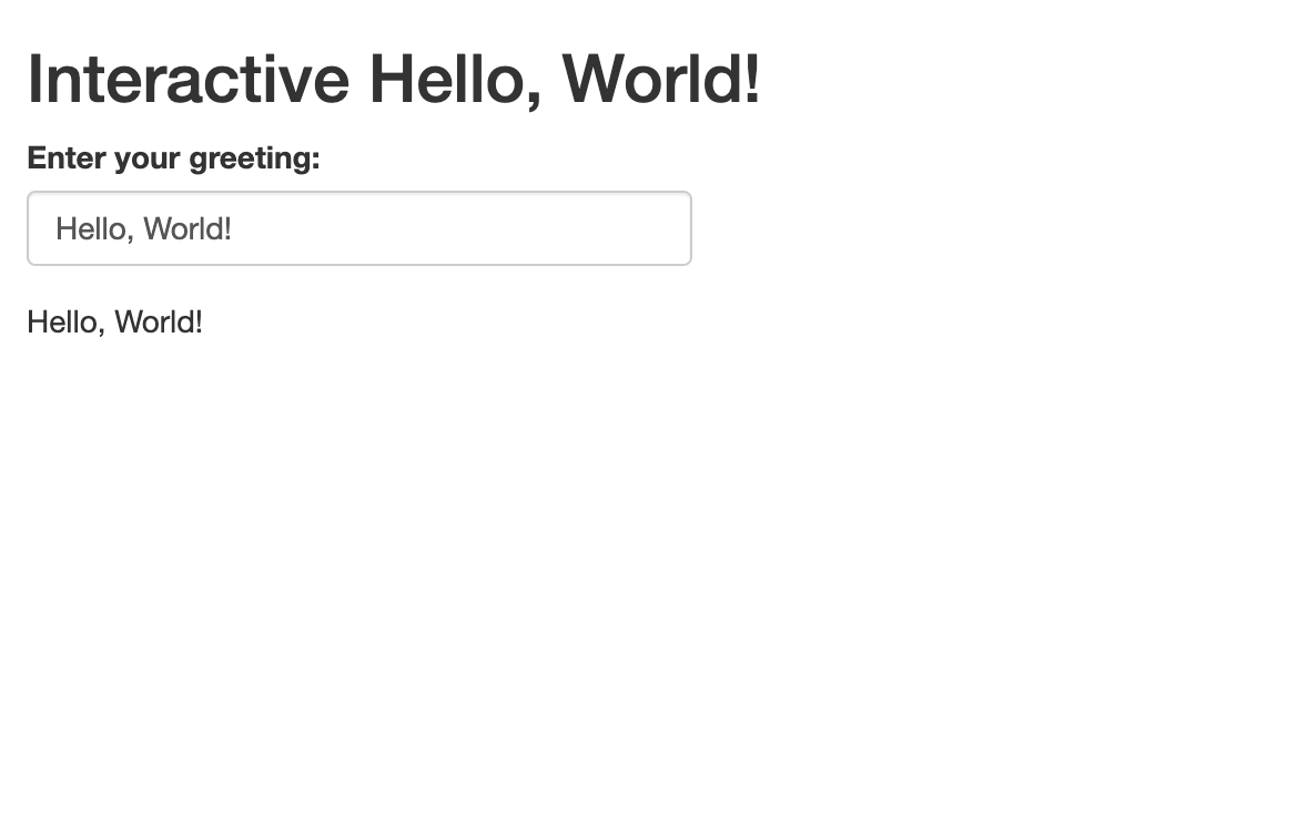
When you run the application, you’ll initially get a result that looks like this:
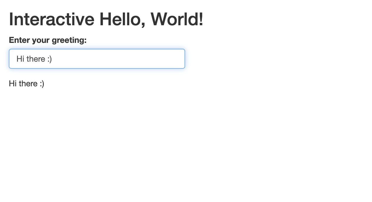
When you change the value in the text box, the output text will also change. For example, if we go ahead and change the greeting in the text box to “Hi there :)”, this change will be reflected in the output:
Let’s now tweak this “greeting” application, which will help you
become familiar with another input function, and get some more practice
writing reactive code. In particular, instead of letting users write any
text they wish into the text box, let’s modify the app to invite users
to select a greeting from a drop-down menu that presents a few different
greetings to choose from; the chosen greeting will be printed as the
output. We can keep all aspects of the code for the initial greeting
application the same; we just have to change the input function from
textInput() (which creates a text box) to
selectInput() which creates a drop-down menu with choices
defined within one of the function’s arguments. For more information,
check the selectInput() function’s documentation. The
modified code will look something like this:
R
# UI: Layout and inputs/outputs go here
ui <- fluidPage(
  titlePanel("Greeting Application"),

  # Input: Dropdown menu for user to select a greeting
  selectInput(
    inputId = "user_input",
    label = "Choose your greeting:",
    choices = c("Hello, World!", "Hi there :)", "What's up?", "Nice to meet you"),
    selected = "Hello, World!"
  ),

  # Output: Display the selected greeting
  textOutput(outputId = "greeting")
)

# Server: Logic and reactivity go here
server <- function(input, output) {

  # Reactive output based on selected greeting
  output$greeting <- renderText({
    input$user_input  # Display the selected greeting
  })
}

# Launch the app
shinyApp(ui, server)
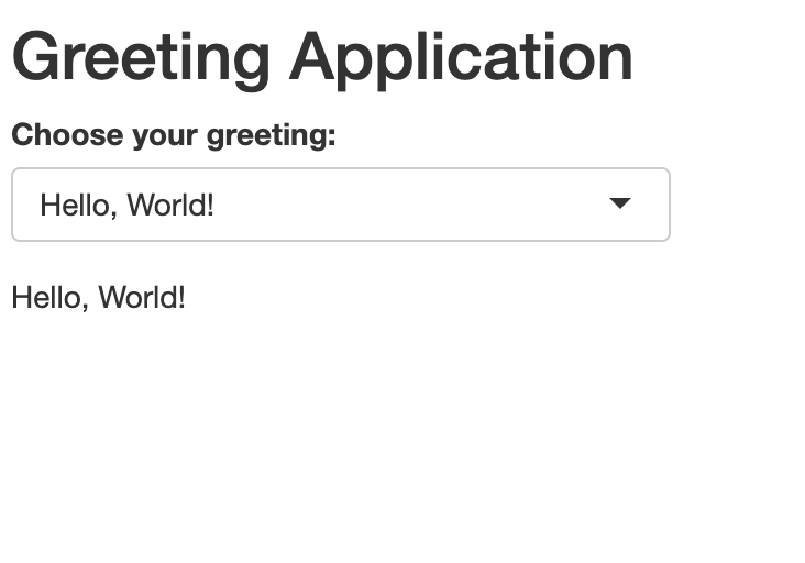
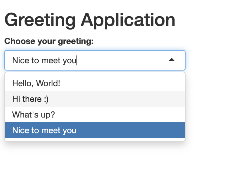
When it is launched, the app looks something like this:
The user can select the desired greeting from the drop-down menu; let’s say they want the “Nice to meet you” greeting:
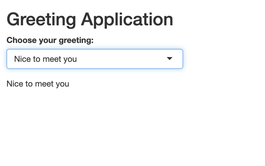
After the selection is made, the corresponding text is printed as text output:
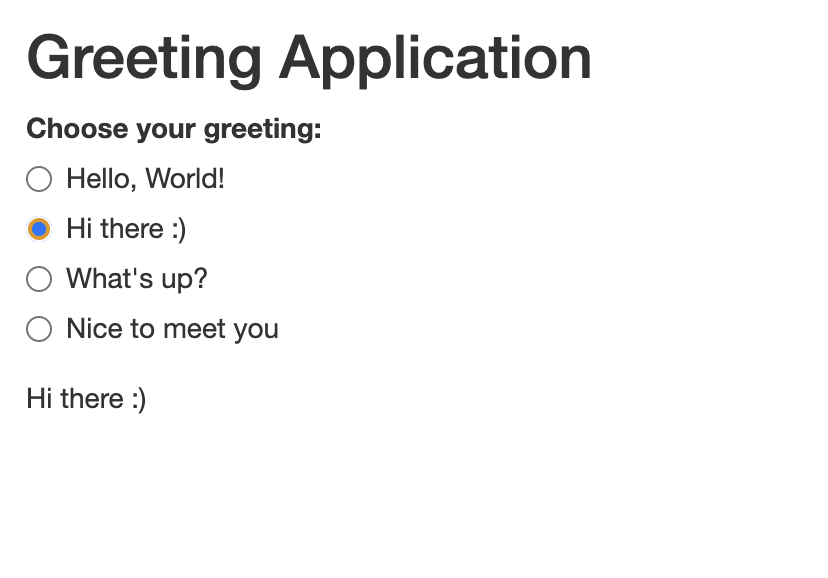
To make this change, you can replace selectInput() with
radioButtons(), while keeping the remaining code unchanged.
It will look something like this:
R
# UI: Layout and inputs/outputs go here
ui <- fluidPage(
  titlePanel("Greeting Application"),

  # Input: Radio buttons for user to select a greeting
  radioButtons(
    inputId = "user_input",
    label = "Choose your greeting:",
    choices = c("Hello, World!", "Hi there :)", "What's up?", "Nice to meet you"),
    selected = "Hello, World!"
  ),

  # Output: Display the selected greeting
  textOutput(outputId = "greeting")
)

# Server: Logic and reactivity go here
server <- function(input, output) {

  # Reactive output based on selected greeting
  output$greeting <- renderText({
    input$user_input
  })
}

# Launch the app
shinyApp(ui, server)
Once launched, the modified application will look something like this:
Let’s now create a slightly different greeting app in which the user provides their name, and the application responds with a personal greeting. We can develop this application with some now-familiar functions:
R
# UI
ui <- fluidPage(
  titlePanel("Personal Greeting App"),

  # Text input for the user's name
  textInput(inputId="name", label="What is your name?"),

  # Output: Greeting text
  textOutput(outputId="greeting")
)

# Server
server <- function(input, output) {
  output$greeting <- renderText({
    paste0("Hello, ", input$name, "! Nice to meet you.")
  })
}

# Run the app
shinyApp(ui = ui, server = server)
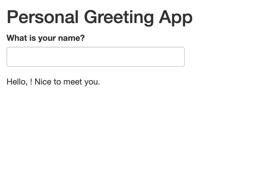
When you launch the application, it looks something like this:
When a name is typed into the text box, the output updates accordingly:
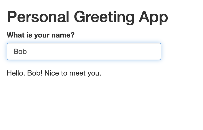
One potential design limitation of this simple application is that
before the name is entered into the text box, the output “Hello, ! Nice
to meet you.” looks awkward. It may be desirable to hide this output
before the name is entered, and only show the complete output once the
name is actually entered into the box. We can accomplish this by
inserting the conditional statement
if (input$name == "") return(NULL) in the
renderText() function before the paste0()
function. This essentially says “If the name field is blank, do not
return an output.” The modified script looks like this:
R
# UI
ui <- fluidPage(
  titlePanel("Personal Greeting App"),

  # Text input for the user's name
  textInput(inputId="name", label="What is your name?"),

  # Output: Greeting text
  textOutput(outputId="greeting")
)

# Server
server <- function(input, output) {
  output$greeting <- renderText({
   if (input$name == "") return(NULL)
    paste0("Hello, ", input$name, "! Nice to meet you.")
  })
}

# Run the app
shinyApp(ui = ui, server = server)
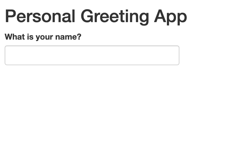
Now, when we launch the app, we’ll see an interface that looks like this:
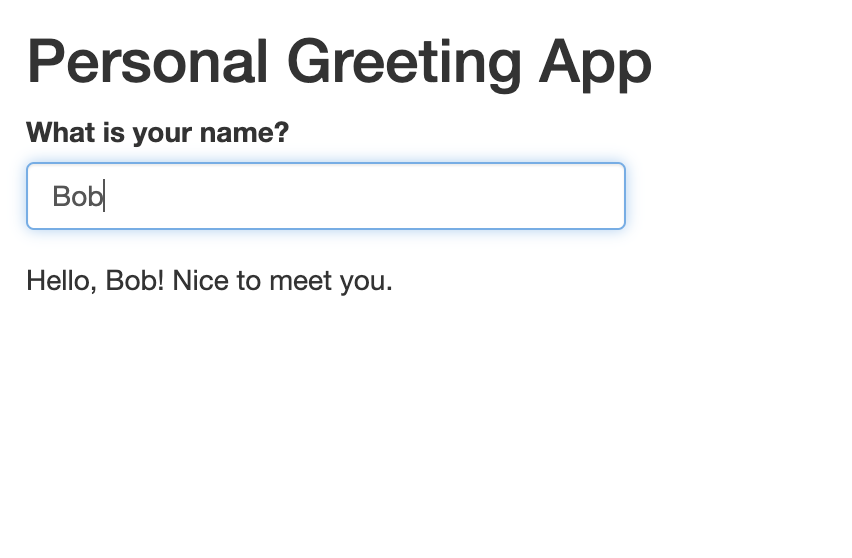
The application will return the full output in response to the user entering their name in the text field:
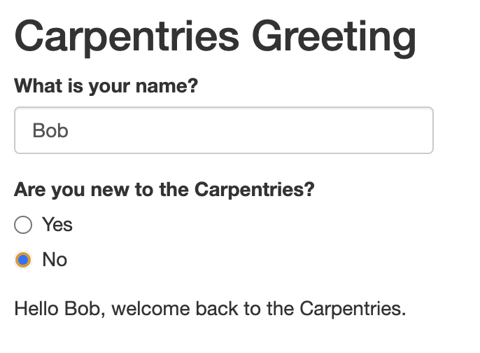
Let’s build on this to make a slighly more complex personal greeting
application. In particular, we’ll write an application that requests two
different inputs from the user, using two different methods. We’ll ask
the user their name, which they’ll supply in a text box. We’ll also ask
the user if this is their first Carpentries workshop, which they’ll
answer by filling in a radio button (Yes/No). If it is their first
Carpentries workshop, the following text output is returned: “Hello,
This interactive application is more complex than the others we’ve
written so far, but uses techniques and functions we’re already familiar
with. The UI includes two input functions, textInput() and
radioButtons that are referenced in the server, within
conditional statements in the renderText() function:
R
# UI
ui <- fluidPage(
  titlePanel("Carpentries Greeting"),

  # Ask for user's name
  textInput(inputId = "name", label="What is your name?"),

  # Ask if they're new
  radioButtons(inputId = "new",
               label = "Are you new to the Carpentries?",
               choices = c("Yes", "No"),
                selected = character(0)), # No default selection

  # Display greeting
  textOutput(outputId = "greeting")
)

# Server
server <- function(input, output) {
  output$greeting <- renderText({
     # Don't show anything unless both inputs are filled
    if (input$name == "" || is.null(input$new)) return(NULL)

    # Build greeting based on response
    if (input$new == "Yes") {
      paste0("Hello ", input$name, ", welcome to the Carpentries.")
    } else if (input$new == "No") {
      paste0("Hello ", input$name, ", welcome back to the Carpentries.")
    } else {
      NULL  # If no radio button is selected yet
    }
  })
}

# Run the app
shinyApp(ui = ui, server = server)
When the resulting app is launched, it looks like this:
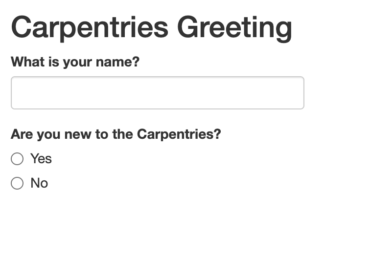
After the user provides their name and clicks the relevant radio button, the text output responds with the appropriate message:
Challenge 4: Explain the logic of the Carpentries greeting app in your own words
Work with a partner, and in your own words, take turns explaining how the application we’ve just written is put together. Focus on input functions, output functions, and the server logic.
Here is a sample explanation: This Shiny app has two main parts: the
UI (user interface) and the server (logic). In the UI, we use
textInput() to ask the user for their name and
radioButtons() to ask whether they are new to the
Carpentries. We set selected = character(0) in the radio
button to ensure that no option is selected by default. We also include
textOutput() as a placeholder where the final greeting
message will appear.
In the server function, we use renderText() to generate
the greeting based on the user’s input. Inside
renderText(), the line
if (input$name == "" || is.null(input$new)) return(NULL)
plays an important role: it tells the app to hold off on showing any
message until both the name and the radio button response are provided.
The input$name == "" part checks whether the name text box
is empty. The is.null(input$new) part checks whether the
user has not yet selected a radio button. The || means “or”
— so if either of these conditions is true, the function returns NULL
(i.e., nothing is shown). Once both inputs are present, the app uses
paste0() to construct a personalized greeting, depending on
whether the user selected “Yes” or “No”, and displays it using the
textOutput() placeholder.
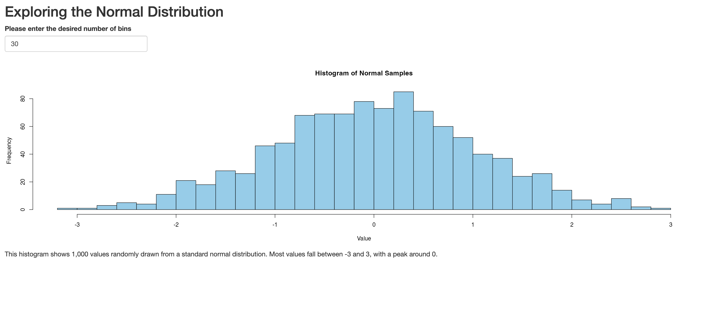
Interactive Plot Applications
Having explored several interactive variations on our static “Hello,
World!” application, let’s now turn to our static plot application
above, and turn it into an interactive application using Shiny’s
reactive functions. Let’s modify the code we used to create the static
plot, and use reactive input functions to allow users to specify the
number of bins in the histogram. To do so, we’ll use
numericInput() within the UI, which gives users a text box
in which they can specify the desired number of bins; in the server,
we’ll replace the number 30 with input$desired_bins, which
sets the “breaks” argument equal to the number specified by the user
(using dollar sign notation to reference this number using the
numericInput function’s input ID):
R
# UI: Layout and inputs/outputs go here
ui <- fluidPage(
  # Add UI code (specifying application's inputs, outputs, and layouts) here
  titlePanel("Exploring the Normal Distribution"),
  numericInput(inputId = "desired_bins",
               label="Please enter the desired number of bins",
               value=30),
  plotOutput(outputId = "normal_plot"),
  textOutput(outputId="context_discussion")
)

# Server: Logic and reactivity go here
server <- function(input, output) {
  # Add server code (specifying application's content) here

  # creates text output
  output$context_discussion<-renderText({
    "This histogram shows 1,000 values randomly drawn from a standard normal distribution. Most values fall between -3 and 3, with a peak around 0."
  })

  # creates plot output
  output$normal_plot<-renderPlot({
    # create vector
    samples <- rnorm(1000, mean = 0, sd = 1)

    # make a histogram of "samples" data
    hist(samples, breaks = input$desired_bins, col = "skyblue",
         main = "Histogram of Normal Samples",
         xlab = "Value")
  })
}

# Launch the app
shinyApp(ui, server)
When we launch the application, we see a numeric textbox with the default value set to 30 (the number of bins we had in our static application):
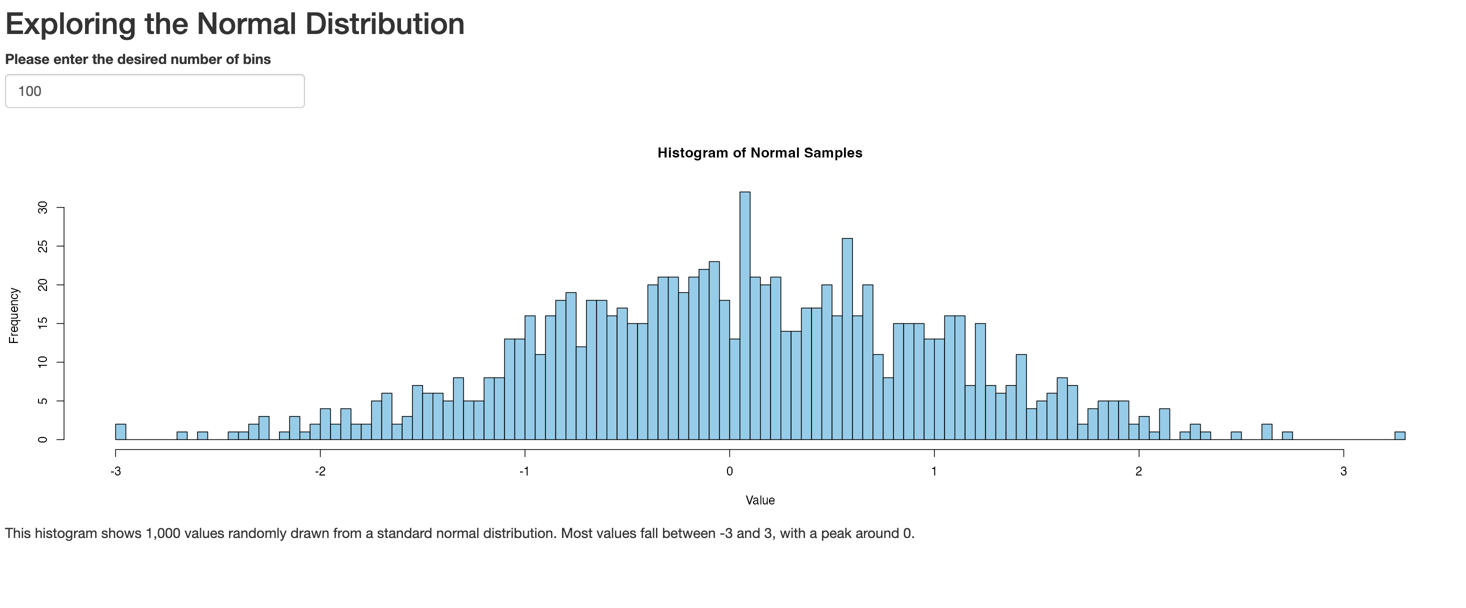
However, the desired number of bins can now be changed by the user, and the plot will respond accordingly. For example, let’s change the number of bins to 100:
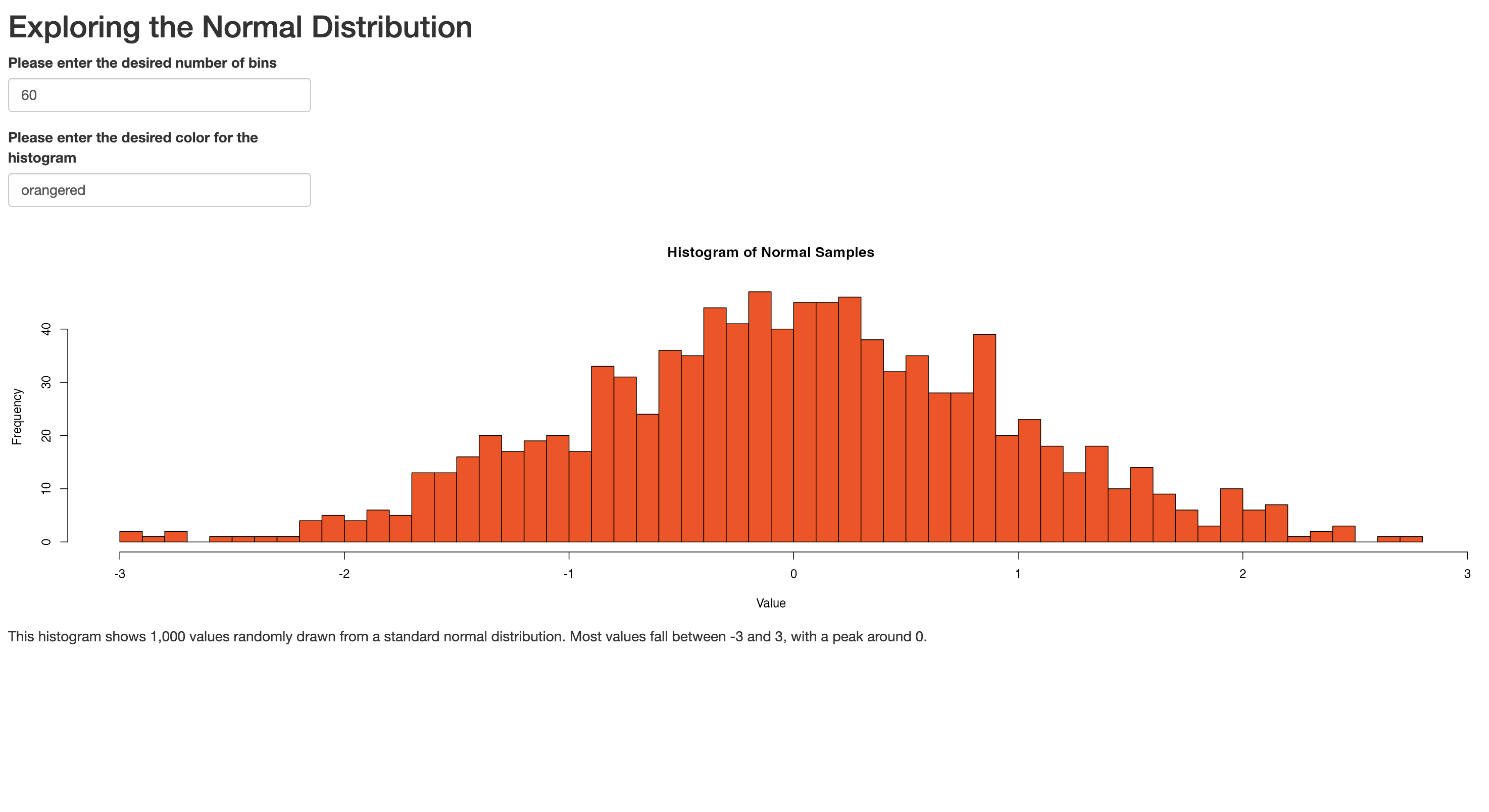
Let’s add another interactive dimension to this application by
allowing users to change the color of the plot. We’ll create a text
input field where a user can type in a color, based on color
codes used in R. We’ll place this text box below the numeric input
box, and create it using the textInput() function; we’ll
refer back to the user specified color in the server using dollar sign
notation in conjunction with the ID argument passed to
textInput():
R
# UI: Layout and inputs/outputs go here
ui <- fluidPage(
  # Add UI code (specifying application's inputs, outputs, and layouts) here
  titlePanel("Exploring the Normal Distribution"),
  numericInput(inputId = "desired_bins",
               label="Please enter the desired number of bins",
               value=30),
  textInput(inputId="desired_color",
            label="Please enter the desired color for the histogram",
            value="skyblue"),
  plotOutput(outputId = "normal_plot"),
  textOutput(outputId="context_discussion")
)

# Server: Logic and reactivity go here
server <- function(input, output) {
  # Add server code (specifying application's content) here

  # creates text output
  output$context_discussion<-renderText({
    "This histogram shows 1,000 values randomly drawn from a standard normal distribution. Most values fall between -3 and 3, with a peak around 0."
  })

  # creates plot output
  output$normal_plot<-renderPlot({
    # create vector
    samples <- rnorm(1000, mean = 0, sd = 1)

    # make a histogram of "samples" data
    hist(samples, breaks = input$desired_bins, col = input$desired_color,
         main = "Histogram of Normal Samples",
         xlab = "Value")
  })
}

# Launch the app
shinyApp(ui, server)
Let’s launch the app, set the number of bins to 60, and the color to “orangered”. It will look something like this:
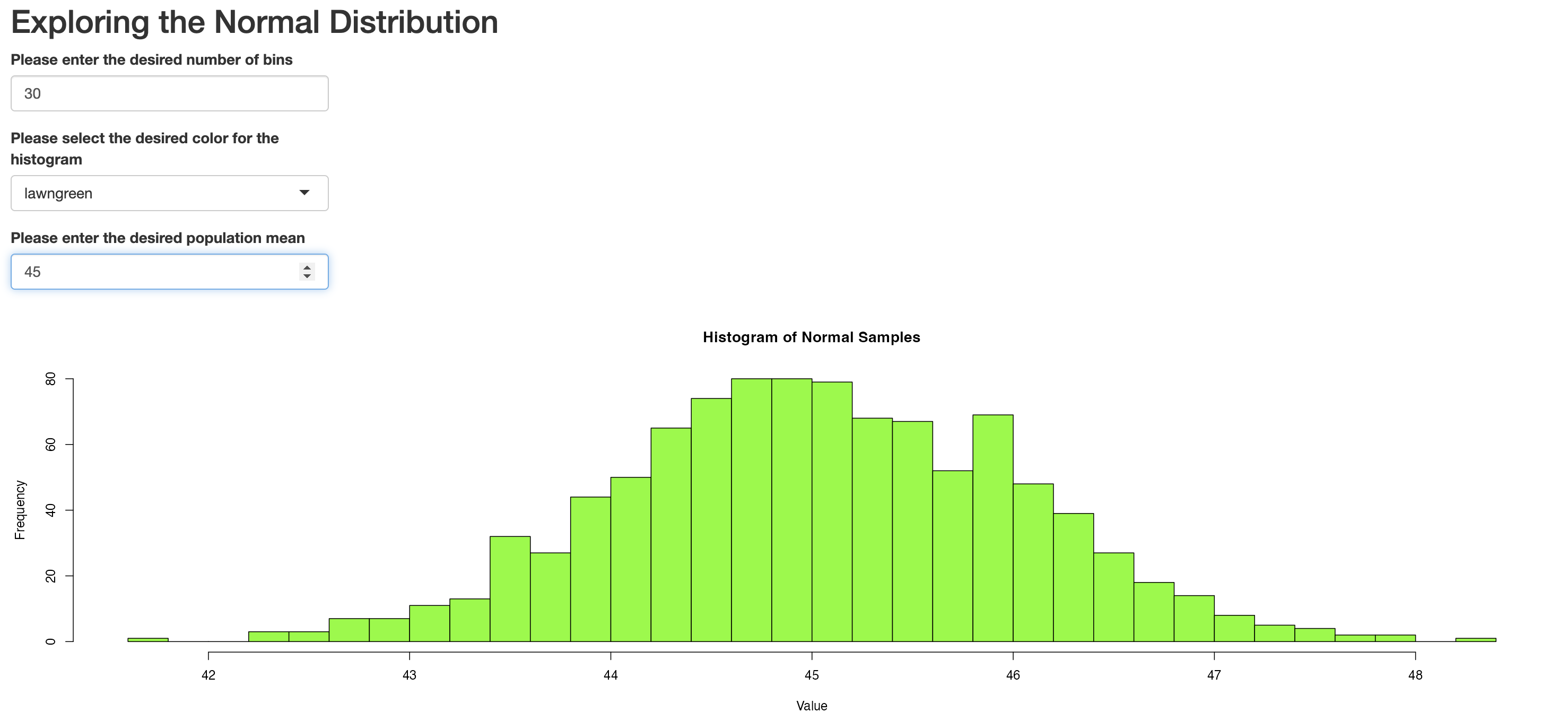
Challenge 5: Modify the interactive plot application
Modify the interactive plot application in the following ways:
- Instead of inviting users to specify their desired color in a textbox, constrain their choices by asking them to select one of the following colors from a dropdown menu: skyblue, orangered, violet, lightcyan, or lawngreen.
- Remove the contextual discussion (i.e. “This histogram shows…)
- Create a numeric input field where users can specify a desired mean for the sample.
Your script should look something like this:
R
# UI: Layout and inputs/outputs go here
ui <- fluidPage(
  # Add UI code (specifying application's inputs, outputs, and layouts) here
  titlePanel("Exploring the Normal Distribution"),
  numericInput(inputId = "desired_bins",
               label="Please enter the desired number of bins",
               value=30),
  selectInput(inputId="desired_color",
            label="Please select the desired color for the histogram",
            choices=c("skyblue", "orangered", "violet", "lightcyan", "lawngreen")),
  numericInput(inputId="desired_mean", label="Please enter the desired population mean", value=0),
  plotOutput(outputId = "normal_plot"),
)

# Server: Logic and reactivity go here
server <- function(input, output) {
  # Add server code (specifying application's content) here

  # creates plot output
  output$normal_plot<-renderPlot({
    # create vector
    samples <- rnorm(1000, mean = input$desired_mean, sd = 1)

    # make a histogram of "samples" data
    hist(samples, breaks = input$desired_bins, col = input$desired_color,
         main = "Histogram of Normal Samples",
         xlab = "Value")
  })
}

# Launch the app
shinyApp(ui, server)
Once the app is launched, if we were to set the number of bins to 100, select “lawngreen” as the color, and choose a mean of 45, we will get something that looks like the following:
Layouts and Themes
We’ll use the app you just created in the exercise above to explore some basic tools that can be used to lay out the elements within your application, as well as style the application as a whole.
Sidebar layouts
First, note that the user inputs in the app you created were laid out on top of the plot. Often, it can be preferable to situate these elements towards the side. Indeed, one of the most useful Shiny application layouts is known as the sidebar layout, in which there is a sidebar for inputs, and a “main” panel for outputs. To see how the sidebar layout works, let’s wrap the application we wrote in the previous exercise into a sidebar layout, with the inputs on the side, and the plot in the main panel:
R
ui <- fluidPage(
  # Add UI code (specifying application's inputs, outputs, and layouts) here
  titlePanel("Exploring the Normal Distribution"),

  sidebarLayout(
    sidebarPanel(
      numericInput(inputId = "desired_bins",
                   label = "Please enter the desired number of bins",
                   value = 30),

      selectInput(inputId = "desired_color",
                  label = "Please select the desired color for the histogram",
                  choices = c("skyblue", "orangered", "violet", "lightcyan", "lawngreen")),

      numericInput(inputId = "desired_mean",
                   label = "Please enter the desired population mean",
                   value = 0)
    ), # closes sidebarPanel

    mainPanel(
      plotOutput(outputId = "normal_plot")
    ) # closes mainPanel
  ) # closes sidebarLayout
) # closes fluidPage


# Server: Logic and reactivity go here
server <- function(input, output) {
  # Add server code (specifying application's content) here

  # creates plot output
  output$normal_plot <- renderPlot({
    # create vector
    samples <- rnorm(1000, mean = input$desired_mean, sd = 1)

    # make a histogram of "samples" data
    hist(samples, breaks = input$desired_bins, col = input$desired_color,
         main = "Histogram of Normal Samples",
         xlab = "Value")
  })
}

# Launch the app
shinyApp(ui, server)
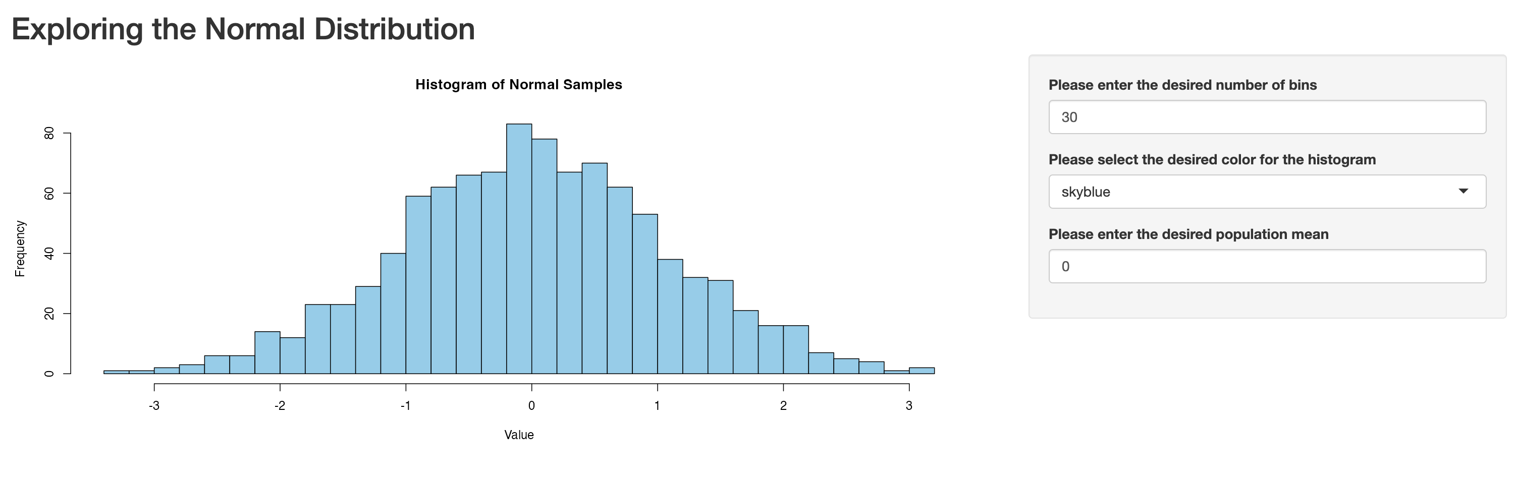
As you can see, the sidebarLayout() function declares a
sidebar structure; within this function, relevant input widgets are
placed within sidebarPanel(), and the outputs to be
displayed within the main panel are placed within
sidebarPanel(). Once this sidebar structure is in place,
the revised app will look like the following:
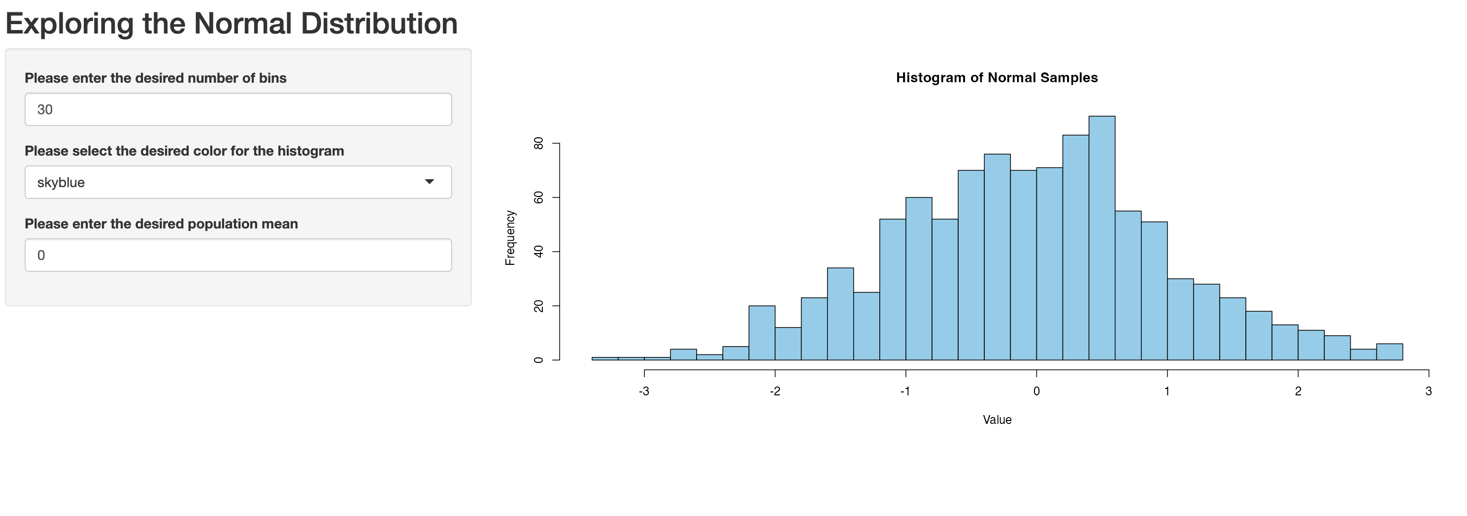
If you wanted to place the input widgets to the right of the main
panel, you can do so by specifying
position="right" withinsidebarLayout(), right before callingsidebarPanel()```.
The modified script would look like this:
R
ui <- fluidPage(
  # Add UI code (specifying application's inputs, outputs, and layouts) here
  titlePanel("Exploring the Normal Distribution"),

  sidebarLayout(
    position="right",
    sidebarPanel(
      numericInput(inputId = "desired_bins",
                   label = "Please enter the desired number of bins",
                   value = 30),

      selectInput(inputId = "desired_color",
                  label = "Please select the desired color for the histogram",
                  choices = c("skyblue", "orangered", "violet", "lightcyan", "lawngreen")),

      numericInput(inputId = "desired_mean",
                   label = "Please enter the desired population mean",
                   value = 0)
    ), # closes sidebarPanel

    mainPanel(
      plotOutput(outputId = "normal_plot")
    ) # closes mainPanel
  ) # closes sidebarLayout
) # closes fluidPage


# Server: Logic and reactivity go here
server <- function(input, output) {
  # Add server code (specifying application's content) here

  # creates plot output
  output$normal_plot <- renderPlot({
    # create vector
    samples <- rnorm(1000, mean = input$desired_mean, sd = 1)

    # make a histogram of "samples" data
    hist(samples, breaks = input$desired_bins, col = input$desired_color,
         main = "Histogram of Normal Samples",
         xlab = "Value")
  })
}

# Launch the app
shinyApp(ui, server)
Yielding an application with the inputs on the right, as expected:
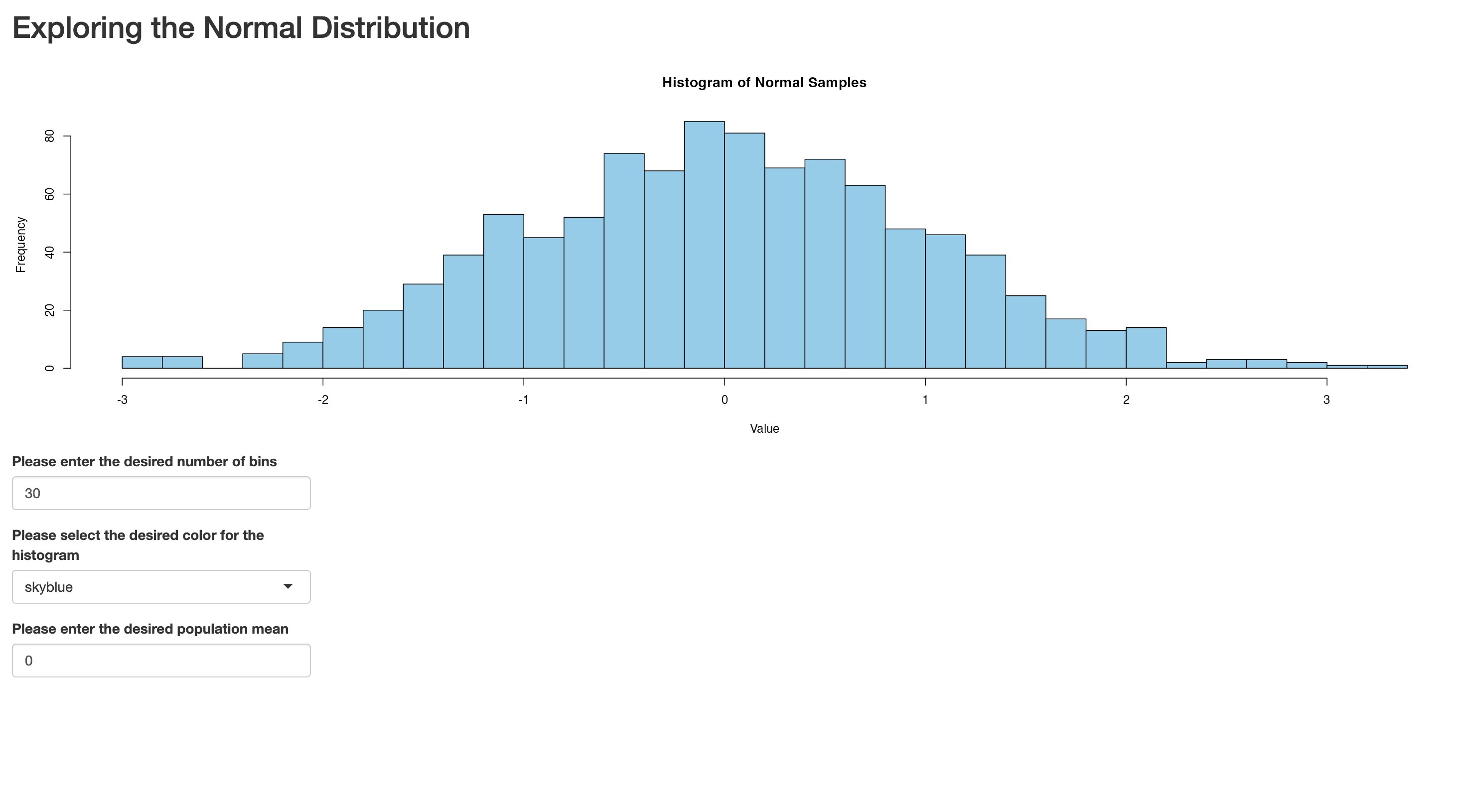
Recall, from above, that if we want the input widgets below the main plot, we could remove the sidebar layout, and place the input widgets below the plot output in the UI:
R
# UI: Layout and inputs/outputs go here
ui <- fluidPage(
  # Add UI code (specifying application's inputs, outputs, and layouts) here
  titlePanel("Exploring the Normal Distribution"),
  plotOutput(outputId = "normal_plot"),
  numericInput(inputId = "desired_bins",
               label="Please enter the desired number of bins",
               value=30),
  selectInput(inputId="desired_color",
            label="Please select the desired color for the histogram",
            choices=c("skyblue", "orangered", "violet", "lightcyan", "lawngreen")),
  numericInput(inputId="desired_mean", label="Please enter the desired population mean", value=0),
)

# Server: Logic and reactivity go here
server <- function(input, output) {
  # Add server code (specifying application's content) here

  # creates plot output
  output$normal_plot<-renderPlot({
    # create vector
    samples <- rnorm(1000, mean = input$desired_mean, sd = 1)

    # make a histogram of "samples" data
    hist(samples, breaks = input$desired_bins, col = input$desired_color,
         main = "Histogram of Normal Samples",
         xlab = "Value")
  })
}

# Launch the app
shinyApp(ui, server)
This minor adjustment in the UI leads to an app with the following appearance:
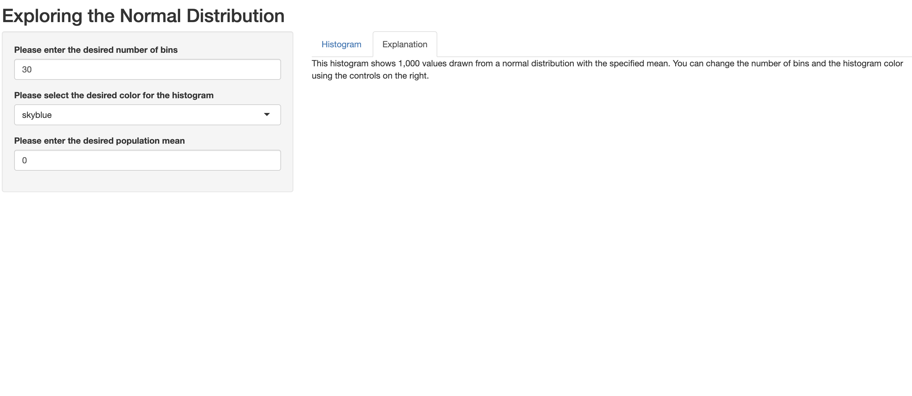
Tabs
So far, our apps have been fairly simple, but as they grow in
complexity and the amount of information displayed increases, it can be
helpful to use tabs as an organizational tool. Tabs allow us to
distribute content across multiple panels, reducing clutter and creating
a more streamlined and user-friendly design. In Shiny, we can use the
tabsetPanel() function to organize the content into tabs.
Each individual tab is then defined using the tabPanel() function, where
the material for that tab is placed. Below, we demonstrate the use of
tabs by placing the plot in one tab (the tab is named “Histogram”), and
then place some contextual information in another tab (named
“Explanation”).
R
# UI
ui <- fluidPage(
  titlePanel("Exploring the Normal Distribution"),

  sidebarLayout(
    sidebarPanel(
      numericInput(inputId = "desired_bins",
                   label = "Please enter the desired number of bins",
                   value = 30),

      selectInput(inputId = "desired_color",
                  label = "Please select the desired color for the histogram",
                  choices = c("skyblue", "orangered", "violet", "lightcyan", "lawngreen")),

      numericInput(inputId = "desired_mean",
                   label = "Please enter the desired population mean",
                   value = 0)
    ), # closes sidebarPanel

    mainPanel(
      tabsetPanel(
        tabPanel(title="Histogram",
                 plotOutput(outputId = "normal_plot")),
        tabPanel(title="Explanation",
                 textOutput(outputId = "context_discussion"))
      ) # closes tabsetPanel
    ) # closes mainPanel
  ) # closes sidebarLayout
) # closes fluidPage

# Server
server <- function(input, output) {

  output$normal_plot <- renderPlot({
    samples <- rnorm(1000, mean = input$desired_mean, sd = 1)

    hist(samples, breaks = input$desired_bins, col = input$desired_color,
         main = "Histogram of Normal Samples",
         xlab = "Value")
  })

  output$context_discussion <- renderText({
    "This histogram shows 1,000 values drawn from a normal distribution with the specified mean.
    You can change the number of bins and the histogram color using the controls on the right."
  })
}

# Run the app
shinyApp(ui = ui, server = server)
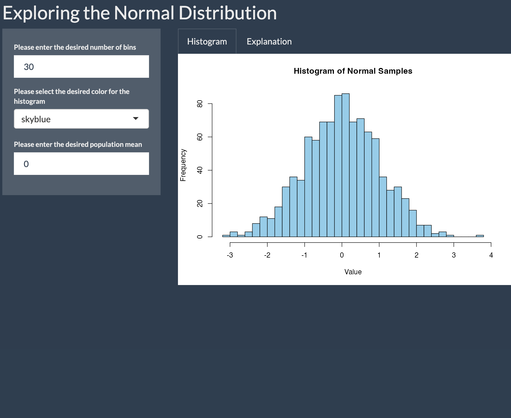
When launched, this tab-based app looks something like this; note the “Histogram” tab is live:

When the user toggles to the “Explanation” tab, it looks like this:
Themes
Issues of application design and style are complex issues, and many
of them are beyond the scope of our Workshop. However, we will briefly
introduce themes, which can help shape the visual appearance of your
applications with relatively little effort. Shiny themes come from the
shinythemes package, and you can add a theme to your app with
one line of code. Before deciding on a theme, you’d probably want to
preview various options, which you can do with the
themeSelector() function. Let’s explore various themes that
could be applied to the tab-based app we made above:
R
# UI
ui <- fluidPage(
  themeSelector(),
  titlePanel("Exploring the Normal Distribution"),
  sidebarLayout(
    sidebarPanel(
      numericInput(inputId = "desired_bins",
                   label = "Please enter the desired number of bins",
                   value = 30),

      selectInput(inputId = "desired_color",
                  label = "Please select the desired color for the histogram",
                  choices = c("skyblue", "orangered", "violet", "lightcyan", "lawngreen")),

      numericInput(inputId = "desired_mean",
                   label = "Please enter the desired population mean",
                   value = 0)
    ), # closes sidebarPanel

    mainPanel(
      tabsetPanel(
        tabPanel(title="Histogram",
                 plotOutput(outputId = "normal_plot")),
        tabPanel(title="Explanation",
                 textOutput(outputId = "context_discussion"))
      ) # closes tabsetPanel
    ) # closes mainPanel
  ) # closes sidebarLayout
) # closes fluidPage

# Server
server <- function(input, output) {

  output$normal_plot <- renderPlot({
    samples <- rnorm(1000, mean = input$desired_mean, sd = 1)

    hist(samples, breaks = input$desired_bins, col = input$desired_color,
         main = "Histogram of Normal Samples",
         xlab = "Value")
  })

  output$context_discussion <- renderText({
    "This histogram shows 1,000 values drawn from a normal distribution with the specified mean.
    You can change the number of bins and the histogram color using the controls on the right."
  })
}

# Run the app
shinyApp(ui = ui, server = server)
When you launch this app, it will launch with a drop-down menu that allows you to select and preview how various themes look in the context of your app:

After previewing the various themes, let’s say you decide you want to
select the “slate” theme. To apply that theme, replace
themeSelector() in the code with
theme=shinytheme("superhero"):
R
# UI
ui <- fluidPage(
  theme=shinytheme("superhero"),
  titlePanel("Exploring the Normal Distribution"),
  sidebarLayout(
    sidebarPanel(
      numericInput(inputId = "desired_bins",
                   label = "Please enter the desired number of bins",
                   value = 30),

      selectInput(inputId = "desired_color",
                  label = "Please select the desired color for the histogram",
                  choices = c("skyblue", "orangered", "violet", "lightcyan", "lawngreen")),

      numericInput(inputId = "desired_mean",
                   label = "Please enter the desired population mean",
                   value = 0)
    ), # closes sidebarPanel

    mainPanel(
      tabsetPanel(
        tabPanel(title="Histogram",
                 plotOutput(outputId = "normal_plot")),
        tabPanel(title="Explanation",
                 textOutput(outputId = "context_discussion"))
      ) # closes tabsetPanel
    ) # closes mainPanel
  ) # closes sidebarLayout
) # closes fluidPage

# Server
server <- function(input, output) {

  output$normal_plot <- renderPlot({
    samples <- rnorm(1000, mean = input$desired_mean, sd = 1)

    hist(samples, breaks = input$desired_bins, col = input$desired_color,
         main = "Histogram of Normal Samples",
         xlab = "Value")
  })

  output$context_discussion <- renderText({
    "This histogram shows 1,000 values drawn from a normal distribution with the specified mean.
    You can change the number of bins and the histogram color using the controls on the right."
  })
}

# Run the app
shinyApp(ui = ui, server = server)
Now, when the app is launched, you’ll see the theme is applied:
Advanced Reactivity
As we noted above, in a reactive programming context, a change in an input (triggered by a user) automatically triggers an update in all downstream outputs that depend on that input. Shiny’s suite of input and output functions, which we are becoming familiar with, facilitate this reactivity, making it possible to develop interactive applications in a relatively straightforward way. Now that we have some more experience in Shiny’s reactive programming context, this section will introduce some more advanced tools and concepts related to reactivity.
Reactive conductors and the reactive() function
In considering reactive programming within Shiny, it’s helpful to distinguish between the following:
- Reactive Sources are the values provided by the user through UI widgets created by input functions
-
Reactive Endpoints are outputs that depend on
reactive sources. These include render functions like
renderText()orrenderPlot(), which respond to input changes and update the UI accordingly. -
Reactive conductors sit in between sources and
endpoints. They are created using the
reactive()function and are used to process or transform input values before they reach the endpoints. They can help reduce code duplication, and improve efficiency.
These reactive conductors are particularly useful when multiple outputs depend on the same derived value. Without a conductor, you’d have to repeat the same calculation in every render function. For example, in a Fahrenheit-to-Celsius conversion app with multiple outputs that display the Celsius temperature in different ways, it would be inefficient to recompute the conversion in each output. Instead, you can use a reactive conductor to perform the conversion once, and then reference it in each render function. This makes your code cleaner, avoids duplication, and improves efficiency.
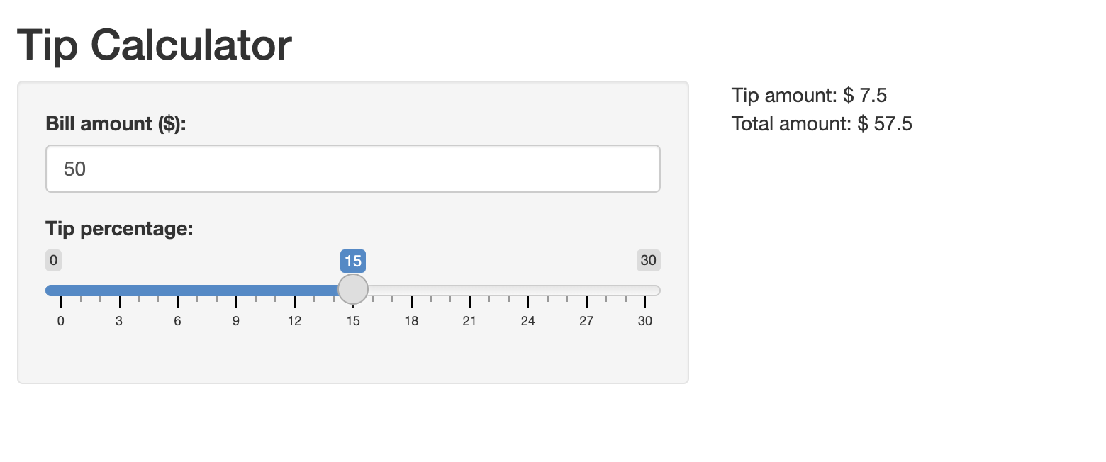
Let’s consider an example. We’ll make a tip calculator application
that takes as input your bill, and the desired tip (as a percentage). It
then returns the dollar value of the tip (based on the bill and desired
tip percentage), and the total value of the bill (including the tip).
Note that in the process we’ll also introduce a new input widget, the
slider bar, which is created with sliderInput():
R
# Define the user interface
ui <- fluidPage(
  titlePanel("Tip Calculator"),  # App title displayed at the top

  sidebarLayout(
    sidebarPanel(  # Sidebar contains input controls
      numericInput("bill", "Bill amount ($):", value = 50, min = 0),  # Input for bill amount
      sliderInput("tip", "Tip percentage:", min = 0, max = 30, value = 15)  # Slider for tip %
    ),

    mainPanel(  # Main panel displays output
      textOutput("tip_amount"),   # Displays computed tip amount
      textOutput("total_amount")  # Displays computed total amount (bill + tip)
    ) # closes mainPanel
  ) # closes sidebarLayout
) # closes fluidPage

# Define the server logic
server <- function(input, output) {

  # Calculate and display the tip amount
  output$tip_amount <- renderText({
    tip_amt <- input$bill * input$tip / 100  # Calculate tip as a percentage of the bill
    paste("Tip amount: $", round(tip_amt, 2))  # Create a string to display the result
  })

  # Calculate and display the total amount
  output$total_amount <- renderText({
    tip_amt <- input$bill * input$tip / 100         # Recalculate tip again (duplicated logic)
    total_amt <- input$bill + tip_amt               # Add tip to bill for total
    paste("Total amount: $", round(total_amt, 2))   # Display total
  })
}

# Run the Shiny app
shinyApp(ui, server)
This yields an application that looks like the following:
The app looks and works as expected, but note that the code used to
create it involved some duplication (which the comments in the code call
attention to). In particular
tip_amt <- input$bill * input$tip / 100 is repeated in
both the tip_amount and total_amount
endpoints. You might wonder why tip_amt can’t be reused
after it’s initially defined in output$tip_amount; the
reason is that the value of tip_amt calculated inside the
first renderText() id local to that block of code. It is
not remembered or shared across other render functions. More generally,
each render function is its own reactive context; variables defined
within one of these contexts only exist there.
Given that’s the case, you might wonder whether you can define a
function in the server to calculate tip_amt, and then use
that function within render functions to avoid code duplication. The
answer is that this won’t work; in particular, regular user-defined
functions are not reactive, so they won’t automatically update when
input values change.
The solution to avoid code duplication of this sort is the
reactive() function. Below, we’ll rewrite the script above,
this time using the reactive() function to calculate
tip_amt, which we’ll then subsequently use in different
endpoints without having to recalculate anything:
R
ui <- fluidPage(
  titlePanel("Tip Calculator"),
  sidebarLayout(
    sidebarPanel(
      numericInput("bill", "Bill amount ($):", value = 50, min = 0),
      sliderInput("tip", "Tip percentage:", min = 0, max = 30, value = 15)
    ),
    mainPanel(
      textOutput("tip_amount"),
      textOutput("total_amount")
    ) # closes mainPanel
  ) # closes sidebarLayout
) # closes fluidPage

server <- function(input, output) {

  # Reactive conductor: compute tip once and reuse it
  tip_amt <- reactive({
    input$bill * input$tip / 100
  })

  output$tip_amount <- renderText({
    paste("Tip amount: $", round(tip_amt(), 2))
  })

  output$total_amount <- renderText({
    total <- input$bill + tip_amt()
    paste("Total amount: $", round(total, 2))
  })
}

shinyApp(ui, server)
Above, tip_amount() is turned into a reactive expression
by being enclosed in reactive() and is subsequently used in
both of the subsequent render functions, which helps avoid code
duplication. Note that when referring to a reactive expression, the name
of the expression must be followed by (), as in
tip_amt().
Consider the benefits of using reactive(), even in this
simple application:
- It avoids duplication and increases efficiency: Tip amount is
calculated once in the
reactive()expression, instead of being repeated in each output block. This can improve app performance, particularly in more complex settings. - Improves maintainability: If you need to change how the tip is calculated, you only need to update it in one place
The ability to define custom reactive conductors with
reactive() is especially useful when creating applications
based on datasets, which we will explore in the next episode. If you are
still a little hazy on what exactly reactive() does or why
it’s useful, it will become clearer then.
Controlling Reactivity with eventReactive()
In the apps we’ve created so far, application outputs automatically update whenever an input changes. Often, however, it can be useful to control or delay reactivity, such that an update only happens when a specific event occurs (such as the user clicking a button). Delaying reactivity in this way can improve a user experience and conserve computational resources.
A useful Shiny function for controlling reactivity in this way is
eventReactive(). Below, we modify the tip calculator
application to only run when the user clicks a button that says
“Calculate Tip”. To do so, we make two changes:
- We include the
actionButton()function in the UI, which creates the button users must click to trigger a calculation - Instead of using
reactive()to calculate the tip, we wrap the calculation ineventReactive(). This tells Shiny to update the tip (and all downstream outputs) only when the Calculate Tip button is clicked.
R
ui <- fluidPage(
  titlePanel("Tip Calculator"),
  sidebarLayout(
    sidebarPanel(
      numericInput("bill", "Bill amount ($):", value = 50, min = 0),
      sliderInput("tip", "Tip percentage:", min = 0, max = 30, value = 15),
      actionButton("calc_btn", "Calculate Tip")
    ),
    mainPanel(
      textOutput("tip_amount"),
      textOutput("total_amount")
    ) # closes mainPanel
  ) # closes sidebarLayout
) # closes fluidPage

server <- function(input, output) {

  # Reactive conductor: compute tip once and reuse it
  tip_amt <- eventReactive(input$calc_btn, {
    input$bill * input$tip / 100
  })

  # create output of tip amount
  output$tip_amount <- renderText({
    paste("Tip amount: $", round(tip_amt(), 2))
  })

  # create output of total amount
  output$total_amount <- renderText({
    total <- input$bill + tip_amt()
    paste("Total amount: $", round(total, 2))
  })
}

shinyApp(ui, server)
When you launch the newly revised application, it will look something like this:
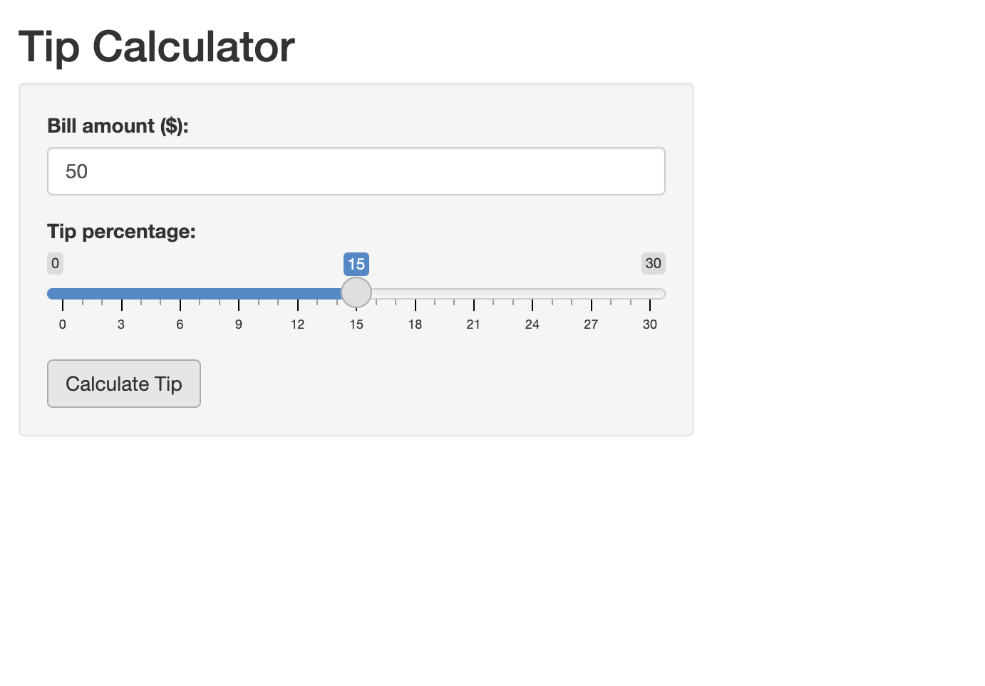
Now, the application will only “run” (i.e. return the relevant outputs) after the user sets the input parameters and clicks the “Calculate Tip” button.
Observers
In Shiny, observers are functions that watch for changes in inputs,
and then trigger actions that don’t directly produce outputs shown in
the app’s user interface, but still affect how the app behaves. These
actions are called “side effects” because they influence the app in ways
other than updating visible output (for example, showing a message,
resetting a form, saving data to a file etc). Unlike reactive
expressions, which calculate values to update the UI, observers don’t
return values. Instead, they simply carry out a task when something
changes. Shiny provides two kinds of observers: observe(),
which runs code whenever any of its inputs change, and
observeEvent(), which waits for a specific event (like a
button click) before running. We can think of observe() and
observeEvent() as counterparts to reactive()
and observeReactive(), but instead of computing values for
outputs, they trigger side effects that change the app’s behavior.
To make this more concrete, let’s see how observe() and
observeEvent() can be used to enrich our tip calculator
app. In particular, we’ll use observe() to grey out the
“Calculate Tip” button if the Bill amount entered by the user is 0.
We’ll also use observeEvent() to reset the input parameters
to their default state when a “Reset” button is clicked; in addition,
when “Reset” is clicked and the input parameters are reset to their
default, the output values in the app are erased; when the “Calculate”
button is clicked again, the output values are once again displayed:
R
ui <- fluidPage(
  useShinyjs(),  # Initialize shinyjs
  titlePanel("Tip Calculator"),
  sidebarLayout(
    sidebarPanel(
      numericInput("bill", "Bill amount ($):", value = 50, min = 0),
      sliderInput("tip", "Tip percentage:", min = 0, max = 30, value = 15),
      actionButton("calc_btn", "Calculate Tip"),
      actionButton("reset_btn", "Reset")
    ),
    mainPanel(
      textOutput("tip_amount"),
      textOutput("total_amount")
    )
  )
)

server <- function(input, output, session) {

  # Reactive conductor: calculate tip when button is clicked
  tip_amt <- eventReactive(input$calc_btn, {
    input$bill * input$tip / 100
  })

  # Disable "Calculate Tip" button when bill is 0
  observe({
    if (input$bill == 0) {
      shinyjs::disable("calc_btn")
    } else {
      shinyjs::enable("calc_btn")
    }
  })

  # create output of tip amount
  output$tip_amount <- renderText({
    paste("Tip amount: $", round(tip_amt(), 2))
  })

  # create output of total amount
  output$total_amount <- renderText({
    total <- input$bill + tip_amt()
    paste("Total amount: $", round(total, 2))
  })

  # Reset form and clear outputs when the "reset" button is clicked
  observeEvent(input$reset_btn, {
    updateNumericInput(session, "bill", value = 50)  # Reset bill to 50
    updateSliderInput(session, "tip", value = 15)    # Reset tip to 15
    shinyjs::hide("tip_amount")                     # Hide tip output
    shinyjs::hide("total_amount")                   # Hide total output
  })

  # Show outputs when "calculate" button is clicked
  observeEvent(input$calc_btn, {
    shinyjs::show("tip_amount")    # Show tip output
    shinyjs::show("total_amount")  # Show total output
  })
}

shinyApp(ui, server)
A couple of points are worth highlighting about these changes to the code.
- You’ll notice that we use functions from the shinyjs
package inside our observers. Shinyjs is a package within the
tidyverse ecosystem that offers a variety of functions that can improve
the user experience. We used the functions
enable()anddisable()to enable or disable the “Calculate Tip” button depending on a condition. We also used it to hide outputs after a user resets the application, and show outputs after a user clicks the “Calculate Tip” button again. - Note the tasks the observers are accomplishing, such as disabling or
enabling buttons or resetting the form to default values. This
underscores our earlier point that observers perform tasks in response
to inputs, and thereby shape the app’s behavior; however, they do not
actually compute values used in outputs (as reactive expressions do).
Note, also, the difference between
observe()andobserveEvent()in action; the former produces its side-effect (i.e. disabling the button) whenever the input value for the bill is 0, while the latter produces its side effects (i.e. resetting the form and clearing or restoring outputs) in response to a specific trigger. - In response to a user clicking the reset button, code within an
observer function hides output, and restores this output when the
“Calculate Tip” button is again clicked. This may seem to contradict our
earlier point, that observers do not actually impact outputs, but
trigger side effects that are relevant for the app’s behavior. It’s
important to note, though, that these “hiding” and “showing” effects
modify the UI’s appearance via JavaScript/CSS (via the shinyjs
functions) rather than altering the reactive values or computations that
drive the outputs, and are therefore best understood as side
effects.
- Note that we included the “session” argument to the server function this time, because of the way in which the side effects of the observer function impact the UI. The details are too technical to get into here, but the basic point is that in apps with multiple concurrent users, the session object ensures that updates (triggered, for example, by the reset button) are applied to the correct user’s instance of the app.
One advanced reactivity function that we won’t cover in detail, but
which you should be aware of, is isolate(). The
isolate() function lets you access an input value without
making your code react to it. In other words, isolate()
lets you use an input while disabling Shiny’s default behavior of
automatically updating outputs in response to input changes. This is
helpful when you want to use an input—like a name or a comment—in your
output, but don’t want changes to that input to automatically rerun your
calculations or update your results. Just like other reactivity
functions, isolate() gives you more control over how and
when your app responds to changes. You’ll want to be aware of
isolate(), particularly if you go on to use Shiny
extensively in the future, and anticipate developing sophisticated
applications; for our purposes now, however, the reactivity functions
we’ve already covered are more fundamental.
Your application code should look something like this:
R
ui <- fluidPage(
  titlePanel("Fahrenheit to Celsius Converter"),
  sidebarLayout(
    sidebarPanel(
      numericInput("temp_f", "Temperature in Fahrenheit:", value = NULL),
      actionButton("convert_btn", "Convert")
    ),
    mainPanel(
      textOutput("result")
    )
  )
)

server <- function(input, output, session) {
  temp_celsius <- eventReactive(input$convert_btn, {
    (input$temp_f - 32) * 5 / 9
  })

  output$result <- renderText({
    paste("Temperature in Celsius:", round(temp_celsius(), 1), "°C")
  })
}

shinyApp(ui, server)
Once the app is launched, it looks something like this:
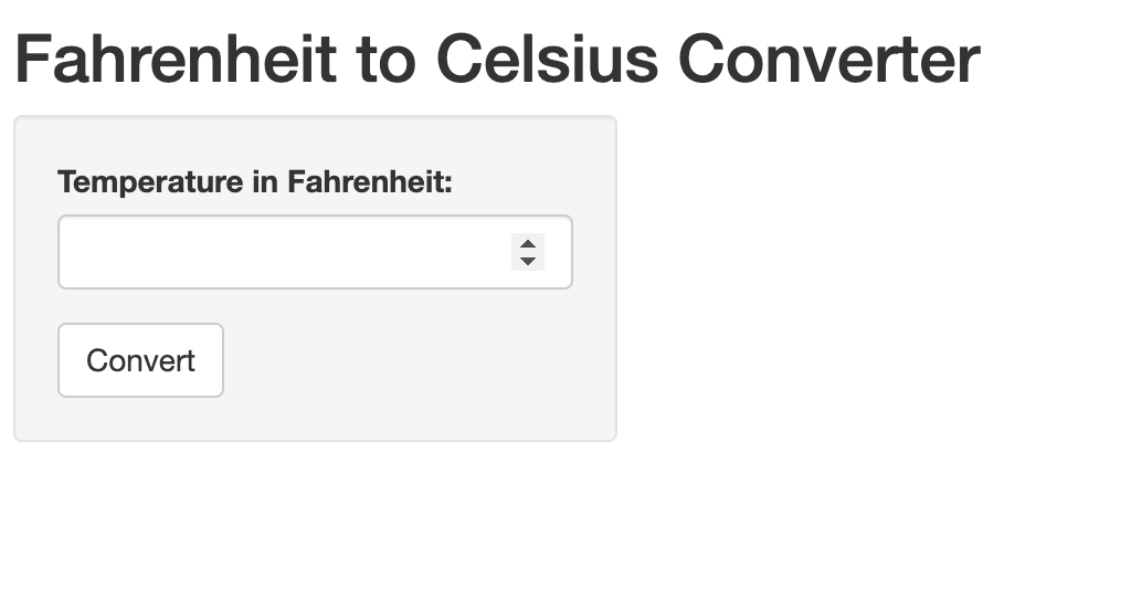
Entering a temperature value in the text box, and then clicking “Convert”, should trigger the application to make the required conversion display the Celsius temperature equivalent.
- The fundamental building blocks of all Shiny applications are the user interface (UI) and the server. Shiny apps are launched by combining the UI and server with the shinyApp() function.
- Output functions serve two purposes: in the UI, they act as placeholders for content; in the server, their corresponding render functions generate content to be displayed. It’s possible to build a static Shiny application using only outputs, without any inputs.
- Input functions create various widgets (such as text boxes, sliders, menus etc.) that allow users to interact with an application by specifying input values. By default, changes in inputs automatically trigger updates in outputs—this behavior is called reactivity. Input values are referenced in the server using their unique IDs.
- Reactive expressions (also known as reactive conductors) created
with
reactive()sit between inputs and outputs, allowing you to process or transform input values before they’re displayed. They help reduce duplication and improve performance. - Observers created with
observe()let you perform side effects—tasks that respond to changes but do not return values (e.g., resetting inputs, enabling/disabling buttons, or saving files). They affect app behavior rather than generating output. - Functions such as
eventReactive()andobserveEvent()provide more control over when reactivity occurs. They are useful for delaying updates until a specific event (like a button click) happens. UseeventReactive()when producing outputs andobserveEvent()for behavior changes that don’t involve rendering output. - Layouts and themes help organize and style your app. Use sidebar layout and tabs to arrange components clearly. Style templates from the shinythemes package can give your app a polished look with minimal effort.