R Foundations: Objects and Data Structures
1 Introduction
In this lesson, we’ll learn some important foundational concepts related to the R programming language. We will discuss R as a calculator, and object assignment, but will spend most of our time learning about three fundamental data structures that you will use all the time when working on applied social science research projects in R: vectors, data frames, and lists.
2 R and R Studio Installation
If you haven’t already, please go ahead and install both the R and RStudio applications. R and RStudio must be installed separately; you should install R first, and then RStudio. The R application is a bare-bones computing environment that supports statistical computing using the R programming language; RStudio is a visually appealing, feature-rich, and user-friendly interface that allows users to interact with this environment in an intuitive way. Once you have both applications installed, you don’t need to open up R and RStudio separately; you only need to open and interact with RStudio (which will run R in the background).
Please follow these instructions to download R and R Studio; make sure you download the version of R appropriate for your operating system.
3 The R Studio Interface
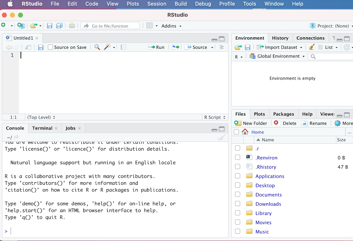
Now that we’ve installed and opened up RStudio, let’s familiarize ourselves with the RStudio interface. When we open up RStudio, we’ll see a window that looks something like this:
If your interface doesn’t look exactly like this, it shouldn’t be a problem; we would expect to see minor cosmetic differences in the appearance of the interface across operating systems and computers (based on how they’re configured). However, you should see four distinct windows within the larger RStudio interface:
- The top-left window is known as the Source window.
- The Source window is where we can write our R scripts (including the code associated with this tutorial), and execute those scripts. We can also type in R code into the “Console” window (bottom-left window), but it is preferable to write our code in a script within the source window. That’s because scripts can be saved (while code written into the console cannot); writing scripts therefore allows us to keep track of what we’re doing, and facilitates the reproducibility of our work. Note that in some cases, we may not see a Source window when we first open RStudio. In that case, to start a new script, simply click the
Filebutton on the RStudio menu bar, scroll down toNew Filebutton, and then selectR Scriptfrom the menu bar that opens up. - It’s also worth noting that the outputs of certain functions will appear in the Source window. In the context of our tutorial, when we want to view our datasets, we will use the
View()function, which will display the relevant data within a new tab in the Source window.
- The Source window is where we can write our R scripts (including the code associated with this tutorial), and execute those scripts. We can also type in R code into the “Console” window (bottom-left window), but it is preferable to write our code in a script within the source window. That’s because scripts can be saved (while code written into the console cannot); writing scripts therefore allows us to keep track of what we’re doing, and facilitates the reproducibility of our work. Note that in some cases, we may not see a Source window when we first open RStudio. In that case, to start a new script, simply click the
- The top-right window is the Environment/History pane of the RStudio interface.
- The “Environment” tab of this window provides information on the datasets we’ve loaded into RStudio, as well as objects we have defined (we’ll talk about objects more later in the tutorial). -The “History” tab of the window provides a record of the R commands we’ve run in a given session.
- The bottom-right window is the Files/Plots/Packages/Help/Viewer window.
- The “Files” tab displays our computer’s directories and file structures and allows us to navigate through them without having to leave the R environment.
- The “Plots” tab is the tab where we can view any visualizations that we create. Within the “Plots” tab, make note of the “Zoom” button, which we can use to enlarge the display of our visualizations if they’re too compressed in the “Plots” window. Also, note the “Export” button within the “Plots” tab (next to the “Zoom” button); we can use this button to export the displayed visualization to a .png or .jpeg file that can be used outside of RStudio.
- The “Packages” tab provides information on which packages have been installed, as well as which packages are currently loaded (more on packages in Sections 2.3 and 2.4 below)
- The “Help” tab displays documentation for R packages and functions. If you want to know more about how a package or function work, we can simply type a “?” followed by the package or function’s name (no space between the question mark and the name) and relevant information will be displayed within the “Help” tab.
- The “Viewer” tab displays HTML output. If we write code that generates an HTML file, we can view it within the “Viewer” tab.
- The bottom-left window is the Console/Terminal/Jobs window.
- The “Console” tab is where we can see our code execute when we run our scripts, as well as certain outputs produced by those scripts. In addition, if there are any error or warning messages, they will be printed to the “Console” tab. We can also type code directly into the console, but as we noted earlier, it is better practice to write our code in a script and then run it from there.
- The “Terminal”, “Jobs” tabs are not relevant for our workshop. We’ll briefly provide an overview of “R Markdown” towards the end of the lesson.
We’re now ready to begin writing some basic code in R. Please go ahead and open up a new script, and follow along by typing the code as we go. To open up a new script, go to File, then click New File, then select R Script.
4 R as a Calculator
At its most basic level, R can be used as a calculator. For instance:
# calculates 2+2
2+2
[1] 4When you type this code out in your script, it should look something like this:
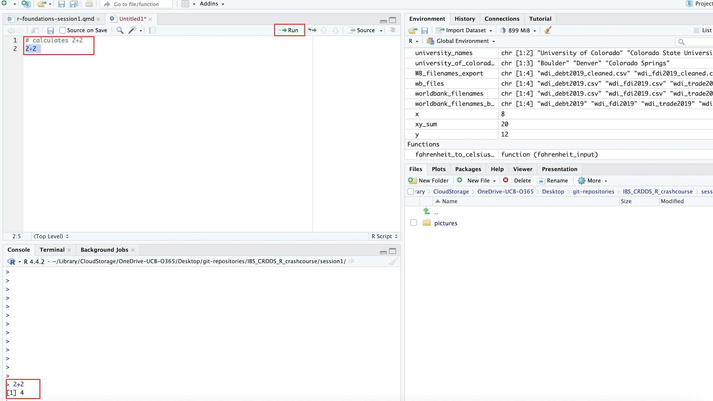
To run the code, you can highlight it and click the Run button (boxed in red). Alternatively, you can place the cursor on the line of code you’d like to run, and use a keyboard shortcut to run the code. On a Mac, the shortcut is clicking Command + Shift + Return. If you are using Windows, the keyboard shortcut to run the current line of code should be Ctrl + Enter.
You should go ahead and save the script in a convenient location by clicking File and then Save As. You should periodically save your work. After you close your R Session, you can always open your saved script, and quickly run the entire script to reproduce your work from prior sessions. To reproduce more than one line of code, or even an entire script, simply highlight the code yoou want to run and click the Run button in the R Studio interface. On a Mac, the shortcut for running all of the code in your script is Cmd + Option + R. On a Windows machine, the shortcut to run the entirety of a script is Ctrl + Shift + Enter.
Before proceeding, one final thing you should note is that the actual code, 2+2, was preceded by a “comment” that was in turn preceded by a #; above, the comment was rather trivial, since it’s fairly self evident what the code was doing. But pretty soon, our code will become more complex and challenging to interpret, and code comments will be an essential way of documenting our work. These comment are an essential way we can communicate with others who might read our code, as well as our future selves. The # sign is always used to introduce a comment, and ensures that any text that comes after it will indeed be interpreted as a comment, rather than as code.
Now, let’s try some more mathematical operations:
# calculates 65 to the power of 4
65^4
[1] 17850625# calculates the sum of 24 and 4, divided by 7
(24+4)/7[1] 4# calculates 2.78 subtracted from 10.453
10.453-2.78[1] 7.673While this is a useful and logical starting point, the possibility of assigning values to objects (or variables) considerably increases the scope of the operations we are able to carry out. We turn to object assignment in the next sub-section.
5 Object Assignment and Manipulation
The concept of object (or variable) assignment is a fundamental concept when working in a scripting environment; indeed, the ability to easily assign values to objects is what allows us to easily and intuitively manipulate and process our data in a programmatic setting. To better understand the mechanics of object assignment, consider the following:
# assign value 5 to new object named x
x<-5
In the code above, we use R’s assignment operator, <- (i.e. a left-pointing arrow) to assign the value 5 to an object named x. Now that an object named x has been created and assigned the value 5, printing x in our console (or printing x in our script and running it) will return the value that has been assigned to the x object, i.e. 5:
# prints value assigned to "x"
x
[1] 5More generally, the process of assignment effectively equates the output created by the code on the right side of the assignment operator (<-) to an object with a name that is specified on the left side of the assignment operator. Whenever we want to look at the contents assigned to an object (i.e. the output created by the code to the right side of the assignment operator), we simply print the name of the object in the R console (or print the name and run it within a script).
Let’s create another object, named y, and assign it the value “12”:
# assign value 12 to new object named y
y<-12
As we noted above, we can print the value that was assigned to y by printing the name of the object:
# prints value assigned to "y"
y
[1] 12Once objects are defined, it’s possible to use those objects in arithmetic operations. For example:
# prints the value of x + y
x+y
[1] 17It’s also possible to use existing objects to assign values to new ones. For example, we can assign the sum of x and y to a new object that we’ll name xy_sum:
# creates a new object, named "xy_sum" whose value is the sum of "x" and "y"
xy_sum<-x+y
Now, let’s print the value of xy_sumthat was created by the previous assignment operation:
# prints value of of "xy_sum"
xy_sum
[1] 17As expected, we see that the value assigned to xy_sum is “17” (i.e. the sum of the values assigned to x and y).
It is possible to change the value assigned to a given object. For example, let’s say we want to change the value assigned to x from “5” to “8”:
# assign value of "8" to object named "x"
x<-8
We can confirm that x is now associated with the value “8”, and the old value has been overwritten:
# prints updated value of "x"
x
[1] 8It’s worth noting that updating the value assigned to x will not automatically update the value assigned to xy_sum (which, recall, is the sum of x and y). If we print the value assigned to xy_sum, note that it is still “17”):
# print value assigned to xy_sum
xy_sum
[1] 17In order for the value assigned to xy_sum to be updated with the new value of x, we must run the assignment operation again, with the updated value of x:
# assigns sum of "y" and newly updated value of "x" to "xy_sum" object
xy_sum<-x+y
Now, the value of xy_sum should reflect the updated value of x, which we can confirm by printing the value of xy_sum:
# prints value of "xy_sum"
xy_sum
[1] 20Note that the value assigned to xy_sum is now “20” (the sum of “8” and “12”), rather than “17” (the sum of “5” and “12”).
Thus far, we’ve been working with numeric values, but it’s also possible to assign non-numeric contents to objects. For example, we can assign strings (i.e. lines of text) to objects. Below, consider the string “Boulder, CO” assigned to an object named our_location:
# assigns string "Boulder, CO" to object named "our_location"
our_location<-"Boulder, CO"
We can print the string that has been assigned to the our_location object by typing the name of the object in our console, or running it from our script:
# prints contents assigned to "our_location" object
our_location
[1] "Boulder, CO"5.1 Naming Objects
While the examples above were very simple, we can assign virtually any R code, and by extension, the data structure(s) generated by that code (such as datasets, vectors, graphs/plots, functions etc.) to an R object. When naming your objects, try to be descriptive, so that the name of the object signifies something about the code or outputs assigned to it.
Note that generally speaking, you have a lot of flexibility in naming your R objects, but there are certain rules. For example, object names must start with a letter, and cannot contain any special symbols (they can only contain letters, numbers, underscores, and periods). Also, object names cannot contain multiple unconnected words; if you’d like to use multiple words or phrases, connect the discrete elements with an underscore (_), or use camel case (where different words are distinguished by beginning each discrete word with a capitalized letter). In addition, there are certain words that are “reserved” for other purposes, and therefore cannot be used in object names (i.e. if, else, TRUE , FALSE, etc).
It is also worth emphasizing that object names are case sensitive; in order to print the contents assigned to an object, that object’s name must be printed exactly as it was created. For example, if we were to type our_Location, we would get an error, since there is no our_Location object (only an our_location object):
# prints contents of "our_Location"
our_Location
Error: object 'our_Location' not foundIn order to keep track of the objects we have created, we can use the handy ls() function, which will print the names of all the objects that are in memory:
# prints objects in memory
ls()
[1] "our_location" "x" "xy_sum" "y" To delete an object from memory, you can pass it to the rm() function. For example, the following will delete the our_location object from memory:
# deletes "our_location" object from memory
rm(our_location)
Now, we can confirm that the our_location object has indeed been deleted by running ls() once again:
# prints objects in memory
ls()
[1] "x" "xy_sum" "y" 6 Data Structures
We now turn to a brief overview of some important data structures that help us to work with data in R. We will consider three data structures that are particularly useful: vectors, data frames, and lists. Note that this is not an exhaustive treatment of data structures in R; there are other structures, such as matrices and arrays, that are also important, and which you may encounter or use in your future work. However, for now, we will limit our discussion to vectors, data frames, and lists, since they are the data structures that are essential for getting started with data-based social scientific research in R, and the data structures that you will likely use most frequently.
6.1 Vectors
In R, a vector is a sequence of values of the same type (i.e. we can have a sequence of numbers or a sequence of strings, but cannot mix and match types in a vector). A vector is created using the c() function. We’ll discuss functions at greater later, but for now you can think of a function as a programmed command that takes input(s), and returns output(s).
For example, let’s make a vector to store the temperatures (in Celsius) of some cities in Asia. The c() function takes as its input a series of numbers, and returns as its output a numeric vector with those numbers as elements:
# makes vector with values 32, 18, 41, 11
c(32, 18, 41, 11)
[1] 32 18 41 11Recall that we can assign vectors to objects with descriptive names. Let’s create a new vector object named asia_temperatures_celsius to store these values:
# assigns vector of temperatures from Asian cities to a new object named "asia_temperatures_celsius"
asia_temperatures_celsius<-c(32, 18, 41, 11)
Now, whenever we want to print the vector assigned to the asia_temperatures_celsius object, we can simply print the name of the object:
# prints contents of "asia_temperatures_celsius"
asia_temperatures_celsius
[1] 32 18 41 11Though we have focused so far on numeric vectors (i.e. vectors where the elements are numbers), it is also possible to create vectors where the elements are strings (i.e. text). For example, let’s create a vector that contains the names of cities that have a University of Colorado campus, and assign it to an object named university_of_colorado_locations
# defines new vector assigned to object named "university_of_colorado_locations" that contains locations of CU campuses
university_of_colorado_locations<-c("Boulder", "Denver", "Colorado Springs")
Now let’s print out its contents:
# prints contents of "university_of_colorado_locations"
university_of_colorado_locations
[1] "Boulder" "Denver" "Colorado Springs"6.2 Vector labels
Sometimes, it can be useful to add text labels to numeric vectors, which can provide important context that helps us to keep track of the information stored within a vector. Let’s return to the asia_temperatures_celsius vector we created above and imagine that the first element in the vector represents the temperature for Mumbai; the second element represents the temperature in Hanoi; the third represents the temperature in Singapore; and the fourth represents the temperature in Beijing. Let’s add these country labels to their corresponding temperature values in the asia_temperatures_celsiusvector. First, we’ll create a vector that contains these text labels and assign it to a new object named country_labels_vector:
# creates country labels vector and assigns it to a new object names "country_labels_vector"
country_labels_vector<-c("Mumbai", "Hanoi", "Singapore", "Beijing")
Now, we’ll use the names() function to assign the labels in country_labels_vector to the temperature values in asia_temperatures_celsius. The first label in country_labels_vector will be assigned to the first temperature value in asia_temperatures_celsius, to indicate that that the temperature of 37 degrees Celsius is associated with Mumbai; the second label in country_labels_vector will be assigned to the second temperature value in asia_temperatures_celsius to indicate that the temperature value of 17 degrees Celsius is associated with Hanoi; and so on.
# uses the "names" function to assign the labels in "country_labels_vector" to the "asia_temperatures_celsius" numeric vector
names(asia_temperatures_celsius)<-country_labels_vector
Now, let’s view the contents of asia_temperatures_celsius, and note that the numeric values are labelled with the text strings contained in country_labels_vector:
# prints updated "asia_temperatures_celsius" vector with labels
asia_temperatures_celsius
Mumbai Hanoi Singapore Beijing
32 18 41 11 It is also possible to add labels to a vector during the process of creating that vector, rather than doing so subsequently; creating labels concurrently with the vector is known as “inline naming”. Below, we create a vector of temperatures in some major North American cities in Celsius using inline naming:
# creates new vector of temperatures in Celsius of major North American cities with labels created using inline naming
north_america_temperatures_celsius<-c("New York City"=25, "Toronto"=15, "Mexico City"=8.5, "Vancouver"=10, "Boston"=12.5)
Let’s print the contents of the newly created north_america_temperatures_celsius vector:
# prints contents of "north_america_temperatures_celsius"
north_america_temperatures_celsius
New York City Toronto Mexico City Vancouver Boston
25.0 15.0 8.5 10.0 12.5 6.3 Indexing, Subsetting, and Modifying Vectors
In many cases, it is useful to subset a vector, and extract specific element(s) from it. Each element in a given vector is assigned an index number, starting with 1; that is, the first element in a vector is assigned an index value of 1, the second element of a vector is assigned an index value of 2, and so on. We can use these index values to extract our desired vector elements. In particular, we can specify the desired index within square brackets after printing the name of the vector object of interest. For example, let’s say we want to extract the 3rd element of the vector in asia_temperature_difference_celsius. We can do so with the following, which returns the temperature value for Singapore, the third element in asia_temperature_difference_celsius:
# Extracts the third element from the "asia_temperatures_celsius" vector
asia_temperatures_celsius[3]
Singapore
41 Since asia_temperatures_celsius has been labelled, it’s also possible to extract vector elements based on their label. For example, instead of extracting Singapore’s temperature with its corresponding index value of three, we can do so with the city label enclosed in quotation marks:
# Extracts the third element from the "asia_temperatures_celsius" vector using its label
asia_temperatures_celsius["Singapore"]
Singapore
41 In some cases, we may want to extract more than one vector element. We can conveniently extract a range of vector elements using their index values.For example, let’s say we want to extract a new vector comprised of the first, second, and third numeric elements in asia_temperatures_celsius; we can do so with the following:
# Extracts elements 1 through 3 in the "asia_temperatures_celsius" and deposits these elements in a new vector
asia_temperatures_celsius[1:3]
Mumbai Hanoi Singapore
32 18 41 Thus far, we have not assigned our subsetted vectors to new objects, but we can easily do so if we want to call those vectors again down the road. Below, for example, we assign the vectors we just subsetted in the last line of code that we ran to a new object named asia_temperatures_subsetted_1to3:
# Extracts elements 1 through 3 in the "asia_temperatures_celsius" and deposits these elements in a new vector assigned to the object "asia_temperatures_subsetted_1to3"
asia_temperatures_subsetted_1to3<-asia_temperatures_celsius[1:3]

# prints contents of "asia_temperatures_subsetted_1to3"
asia_temperatures_subsetted_1to3
Mumbai Hanoi Singapore
32 18 41 We can also use negative index numbers to subset vectors; in particular, while passing a positive index number will extract the vector element that corresponds with that number and creates a new vector with that subsetted element, passing a negative index number will return a vector that deletes the element that corresponds to the the absolute value of the negative index number. For example, the following removes the temperature associated with Hanoi (the second element in asia_temperatures_celsius) and returns a new vector with the remaining temperatures:
# removes second element in "asia_temperatures_celsius" vector and returns a vector with the remaining values
asia_temperatures_celsius[-2]
Mumbai Singapore Beijing
32 41 11 It’s also possible to delete a range of elements in a vector using negative index numbers. Below, for example, we delete the second and third elements from asia_temperatures_celsius and return a vector with the remaining values:
# removes second and third elements in "asia_temperatures_celsius" vector (i.e. the temperatures associated with Hanoi and Singapore) and returns a vector with the remaining temperature values
asia_temperatures_celsius[-2:-3]
Mumbai Beijing
32 11 Sometimes, we may want to subset our vectors by referencing non-consecutive elements. For example, instead of extracting the first through third elements of the asia_temperatures_celsius vector, perhaps we only want to extract the first and third elements, without also extracting the second. Intuitively, we could try the following:
# tries to extract the first and third elements from "asia_temperatures_celsius" and deposit them into a new vector
asia_temperatures_celsius[1,3]
Error in asia_temperatures_celsius[1, 3]: incorrect number of dimensionsHowever, as you can see, this syntax throws an error. Instead, if we want to extract non-continuous elements from a vector, we have to pass the index numbers into their own vector, and enclose this vector of index numbers in square brackets. For example, to extract only the first and third elements from asia_temperatures_celsius, we would do the following:
# extracts the first and third elements from "asia_temperatures_celsius" and deposits them into a new vector
asia_temperatures_celsius[c(1,3)]
Mumbai Singapore
32 41 The same syntax can be used when removing multiple non-consecutive elements; for example, let’s say we want to remove the first and third elements from the asia_temperatures_celsius vector, and create a new subsetted vector with the remaining elements. We can do so with the following:
# Removes the first and third elements from "asia_temperatures_celsius" and makes a new vector with the remaining elements
asia_temperatures_celsius[c(-1,-3)]
Hanoi Beijing
18 11 We can also use this basic syntax to subset multiple vector elements using labels, rather than index numbers. For example:
# extracts temperature values for Mumbai and Singapore and deposits them in a new vector using labels
asia_temperatures_celsius[c("Mumbai", "Singapore")]
Mumbai Singapore
32 41 Though we now have a sense of how to subset vectors, there might be instances in which you want to add new elements to a vector. For example, let’s say that we want to add temperature data (and associated labels) for some other cities to asia_temperatures_celsius. Let’s say we want to add the temperature of Jakarta, which was 32 degrees Celsius, and Manila, which was 26.5 degrees Celsius. We can do so with the following syntax:
# Adds temperatures for Jakarta and Manila to the "asia_temperatures_celsius" vector
asia_temperatures_celsius<-c(asia_temperatures_celsius, "Jakarta"=32, "Manila"=26.5)
In particular, we call the function to make vectors (c()); the first argument is the name of the vector object to which we’re adding elements, and the subsequent arguments are the numeric elements along with their labels. We can confirm that the new elements have been added by printing out the contents of the updated asia_temperatures_celsius vector:
# prints contents of updated "asia_temperatures_celsius" vector
asia_temperatures_celsius
Mumbai Hanoi Singapore Beijing Jakarta Manila
32.0 18.0 41.0 11.0 32.0 26.5 In some cases, we may have two or more vectors that we want to combine into a single, unified vector. For example, let’s say we want to combine our vector of temperatures in Asian cities (asia_temperatures_celsius) with our vector of temperatures in North American cities (north_america_temperatures_celsius). We can do so by passing the name of these vector objects to the c() function; below, we’ll assign this combined vector to a new object named asia_north_america_temperatures_celsius:
# combines "asia_temperatures_celsius" vector and "north_america_temperatures_celsius" into a new combined vector that's assigned to an object named "asia_north_america_temperatures_celsius"
asia_north_america_temperatures_celsius<-c(asia_temperatures_celsius, north_america_temperatures_celsius)
Let’s print the contents of asia_north_america_temperatures_celsius to confirm that the vectors have been combined as expected:
# prints contents of "asia_north_america_temperatures_celsius"
asia_north_america_temperatures_celsius
Mumbai Hanoi Singapore Beijing Jakarta
32.0 18.0 41.0 11.0 32.0
Manila New York City Toronto Mexico City Vancouver
26.5 25.0 15.0 8.5 10.0
Boston
12.5 The basic principles and code we’ve used to subset and modify numeric vectors (i.e. vectors comprised of numeric elements) can be applied to subset and modify character vectors (i.e. vectors comprised of string/text elements). Recall the character vector of University of Colorado locations, university_of_colorado locations. We can use index numbers to extract elements from character vectors in much the same way we do for numeric vectors.
# extracts the second element from "university_of_colorado_locations"
university_of_colorado_locations[2]
[1] "Denver"We can also subset a character vector using index numbers to extract a range of elements:
# extracts the second and third elements from "university_of_colorado_locations"
university_of_colorado_locations[2:3]
[1] "Denver" "Colorado Springs"We could get the same result using a negative index number to delete the first element:
# extracts the second and third elements from "university_of_colorado_locations" using a negative index number to remove the first element
university_of_colorado_locations[-1]
[1] "Denver" "Colorado Springs"We can also combine character vectors. For example, let’s say we have a vector that contains the locations of Colorado State University campuses:
# creates character vector of CSU campus locations and assigns it to a new vector named "colorado_state_university_locations"
colorado_state_university_locations<-c("Fort Collins", "Pueblo")
And we want to combine colorado_state_university_locations with university_of_colorado_locations to form a new character vector. We can do so with the following:
# creates new character vector that combines elements from "university_of_colorado_locations" and "colorado_state_university_locations" and assigns it to a new object named "co_public_university_locations"
co_public_university_locations<-c(university_of_colorado_locations, colorado_state_university_locations)

# prints contents of "co_public_university_locations"
co_public_university_locations
[1] "Boulder" "Denver" "Colorado Springs" "Fort Collins"
[5] "Pueblo" It’s also possible to add labels to character vectors, which can be a useful way of embedding metadata in our character vectors. For example, let’s say we want to add labels to co_public_university_locations indicating whether a location corresponds to a UC or CSU institution. We can do so with the names() unction, as we did with numeric vectors:
# uses the "names" function to assign labels to the "co_public_university_locations" vector elements
names(co_public_university_locations)<-c("UC", "UC", "UC", "CSU", "CSU")

# prints contents of "co_public_university_locations" updated with labels
co_public_university_locations
UC UC UC CSU
"Boulder" "Denver" "Colorado Springs" "Fort Collins"
CSU
"Pueblo" We can use the same procedure we used with numeric vectors to create “inline” (i.e. concurrent) labels. To see this, let’s create a vector with the location of the flagship institutions of the University of Colorado and Colorado State systems, respectively, with labels designating which system the university associated with that location is a part of:
# creates vector of flagship university locations, with labels designating if a location is associated with the UC or CSU flagship
flagship_university_locations<-c(UC="Boulder", CSU="Fort Collins")

# prints contents of "flagship_university_locations"
flagship_university_locations
UC CSU
"Boulder" "Fort Collins" Finally, if we want to add new elements to an existing character vector, we can use the same syntax we used for numeric vectors. The Colorado State University system also includes a Global online university that we didn’t include in our vectors above. Let’s say we want to add CSU-Global to the colorado_state_university_locations vector. We can do so with the following:
# Adds "Global" campus to "colorado_state_university_locations" vector
colorado_state_university_locations<-c(colorado_state_university_locations, "Global")

# prints updated contents of "colorado_state_university_locations"
colorado_state_university_locations
[1] "Fort Collins" "Pueblo" "Global" Let’s say we also want to add the global location to co_public_university_locations with a corresponding label. We can do so with the following:
# adds global location to "co_public_university_locations" along with CSU label
co_public_university_locations<-c(co_public_university_locations, CSU="Global")

# prints updated contents of "co_public_university_locations"
co_public_university_locations
UC UC UC CSU
"Boulder" "Denver" "Colorado Springs" "Fort Collins"
CSU CSU
"Pueblo" "Global" 6.4 Vectorized Operations
Once a vector has been created, it’s possible to carry out operations on its elements; it’s important to briefly get an intuitive sense for how such vector operations work. There are different types of vector operations to be aware of. There are scalar operations, which involve arithmetic operations apply a constant value to every element of a numeric vector (i.e. adding ten to each vector element). It’s also possible to carry out arithmetic operations with more than one vector (i.e. adding two vectors together); such operations are typically known as vector operations. More generally, one of R’s benefits is that it allows us to use vectors to carry out iterative (repeated) operations without using programming constructs such as loops. For example, if you have some data and want to apply a formula or function to all of your data points, you could simply put those data points into a vector, and apply the formula or function to that vector, which will implement the desired operation on each element of the vector. Such operations, along with scalar and vector operations, are collectively referred to as “vectorized operations.”
Let’s first consider scalar operations. Let’s go back to the asia_temperatures_celsius vector and remind ourselves of it its contents:
# prints contents of "asia_temperatures_celsius"
asia_temperatures_celsius
Mumbai Hanoi Singapore Beijing Jakarta Manila
32.0 18.0 41.0 11.0 32.0 26.5 Let’s say that something went wrong in the transcription of temperatures, and all of the temperatures in asia_temperatures_celsius are understated by two degrees. We can add two to each element in the asia_temperatures_celsius vector, and thereby fix the error, with the following scalar operation:
# adds two to each element of "asia_temperatures_celsius" vector
asia_temperatures_celsius+2
Mumbai Hanoi Singapore Beijing Jakarta Manila
34.0 20.0 43.0 13.0 34.0 28.5 Of course, the above operation did not permanently add two to all of the elements in asia_temperatures_celsius, since we did not overwrite the existing vector by assigning the changes back to the object. We can do so with the following:
# adds two to each element of "asia_temperatures_celsius" vector and assigns the changes back to the object
asia_temperatures_celsius<-asia_temperatures_celsius+2
We can now confirm that each of the temperature values in asia_temperatures_celsius have been increased by two:
# prints updated contents of "asia_temperatures_celsius"
asia_temperatures_celsius
Mumbai Hanoi Singapore Beijing Jakarta Manila
34.0 20.0 43.0 13.0 34.0 28.5 Let’s now consider another vectorized operation that’s slightly more complex. Let’s say we want to convert the Celsius temperatures in asia_temperatures_celsius to Fahrenheit values, which are stored in a new asia_temperatures_fahrenheit vector object. We can do so by applying the Celsius to Fahrenheit conversion formula to asia_temperatures_celsius with the following:
# applies the Celsius to Fahrenheit conversion formula to all of the Celsius temperatures in "asia_temperatures_fahrenheit" and assigns the resulting vector of Fahrenheit temperatures to a new object named "asia_temperatures_fahrenheit"
asia_temperatures_fahrenheit<-asia_temperatures_celsius*(9/5)+32
The conversion formula of Celsius*(9/5)+32 is applied to the first element of asia_temperatures_celsius and the result is deposited as the first element in asia_temperatures_fahrenheit; the formula is then applied to the second element of asia_temperatures_celsius and the result is deposited as the second element in asia_temperatures_fahrenheit ; and so on. Let’s take a look at the contents of asia_temperatures_fahrenheit:
# prints contents of "asia_temperatures_fahrenheit"
asia_temperatures_fahrenheit
Mumbai Hanoi Singapore Beijing Jakarta Manila
93.2 68.0 109.4 55.4 93.2 83.3 Though we have been focused thus far on applying changes to a single vector, it is often the case that we may have information stored in multiple numeric vectors, and want to carry out mathematical operations that involves those vectors. For example, recall our vector of temperatures in North America:
# prints contents of "north_america_temperatures_celsius"
north_america_temperatures_celsiusNew York City Toronto Mexico City Vancouver Boston
25.0 15.0 8.5 10.0 12.5 Let’s say we have another vector of North American temperatures for those same cities from a subsequent time period. Below, we’ll create this vector, and assign it to a new object named north_america_temperatures_celsius_B:
# creates vector of temperatures in Celsius for the same North American cities as in the "north_america_temperatures_celsius" vector for a subsequent time period, and assigns the vector to a new object named "north_america_temperatures_celsius_B"
north_america_temperatures_celsius_B<-c("New York City"=27, "Toronto"=11, "Mexico City"=8.5, "Vancouver"=10.5, "Boston"=17)Now, let’s say we want to compute the difference in temperatures across these time frames, and deposit the calculated temperature differences in a new vector. We do so below, assigning the vector of temperature differences to a new object named north_america_temperature_difference:
# Computes the difference between "north_america_temperatures_celsius_B" and "north_america_temperatures_celsius" and assigns the difference to a new object named "north_america_temperature_difference"
north_america_temperature_difference<-north_america_temperatures_celsius_B-north_america_temperatures_celsiusThe code above takes the first element in north_america_temperatures_celsius, subtracts it from the first element in north_america_temperatures_celsius_B, and deposits the difference as the first element in the new north_america_temperature_difference vector; it then takes the second element in north_america_temperatures_celsius, subtracts it from the second element in north_america_temperatures_celsius_B, and deposits the difference as the second element in the new north_america_temperature_difference vector; and so on for the other elements. In short, the corresponding elements of the two vectors are related through the mathematical operation of subtraction; this concept, wherein operations with multiple vectors are applied to the corresponding elements of those vectors, is often referred to as “element-wise operations”.
Given this framework of element-wise operations, it’s important to note what happens when carrying out operations with vectors of unequal length. Let’s create some toy vectors of unequal length and add them together:
# creates two new vectors, "a" and "b" of unequal length
a<-c(3,5,7)
b<-c(6,12,3,5)
a + bWarning in a + b: longer object length is not a multiple of shorter object
length[1] 9 17 10 8The first three element-wise operations are straightforward: 3+6=9, 5+12=17, and 7+3=10. However, a does not have a fourth element, but b does; how is this handled? In short, the shorter vector is “recycled” (i.e. repeated) to match the length of the longer one. In this case, once we hit the end of a the recycling process goes back to the beginning, takes the element “3”, and uses it as the fourth element in the vector, which can be added to the fourth element of b to yield “8” as the fourth element in the resultant a+b vector. Let’s now slightly tweak this scenario by adding another element, “6”, to vector b :
a<-c(3,5,7)
b<-c(6,12,3,5,6)What do you think happens when we carry out a+b? In particular, what do you think are the fourth and fifth elements of a+b? The principle of vector recycling suggests that the fourth element will be 8 (3+5), while the fifth element will be 11 (5+6):
a+bWarning in a + b: longer object length is not a multiple of shorter object
length[1] 9 17 10 8 11Being aware of this property of vectors in R can be helpful in troubleshooting errors or unexpected behavior once you’re working with real-world data in R.
It is also possible to carry out vectorized operations on character vectors that are somewhat analogous to the mathematical operations carried out on numeric vectors. To illustrate one useful example that draws on the paste0() function, let’s first create two character vectors:
# creates vector of university names
university_names<-c("University of Colorado, ", "Colorado State University, ")
# creates vector of locations
locations<-c("Boulder", "Fort Collins")Now, we’ll use the paste() function to carry out an element-wise concatenation of the strings in these two vectors; we’ll assign the resulting vector of concatenated strings to a new object named university_name_location:
# uses paste0 function to paste the strings in "university_names" and "locations" together in element-wise fashion and assign the resulting character vector to "university_name_location"
university_name_location<-paste0(university_names, locations)Let’s go ahead and print the contents of university_name_location:
# prints contents of "university_name_location"
university_name_location[1] "University of Colorado, Boulder"
[2] "Colorado State University, Fort Collins"Vectorized operations with the paste0() can be very useful in creating names for objects and file names when working in applied settings.
6.5 Data Frames
The data frame structure is the workhorse of data analysis in R. A data frame resembles a table, of the sort you might generate in a spreadsheet application.
Often, the most important (and arduous) step in a data analysis workflow is to assemble disparate strands of data into a tractable data frame. What does it mean for a data frame to be “tractable”? One way to define this concept more precisely is to appeal to the concept of “tidy” data, which is often referenced in the data science world. Broadly speaking, a “tidy” data frame is a table in which:
Each variable has its own column
Each observation has its own row
Each value has its own cell
We will work extensively with data frames later in the workshop, but let’s generate a toy data frame from scratch, and assign it to a new object. We will generate a data frame containing made up country-level data on basic economic, geographic, and demographic variables, and assign it to a new object named country_df. The data frame is created through the use of the data.frame() function, which has already been programmed into R. Column names and the corresponding column values are passed to the data.frame() function in the manner below, and the function effectively binds these different columns together into a table:
# Creates a toy country-level data frame
country_df<-data.frame(Country=c("Country A", "Country B", "Country C"),
GDP=c(8000, 30000, 23500),
Population=c(2000, 5400, 10000),
Continent=c("South America", "Europe", "North America"))To observe the structure of the table, we can print it to the R console by simply printing the name of the object to which it has been assigned:
# prints "country_df" data frame to console
country_df Country GDP Population Continent
1 Country A 8000 2000 South America
2 Country B 30000 5400 Europe
3 Country C 23500 10000 North AmericaOne nice feature of R Studio is that instead of simply printing our data frames into the console, we can view a nicely formatted version of our data frame by passing the name of the data frame object through the View() function. For example, the code below will bring up the country_df data frame as a new tab in R Studio:
# pulls up "country_df" data frame in R Studio data viewer
View(country_df)Note the “tidy” features of this simple data frame:
Each of the variables (i.e. GDP, Population, Continent) has its own column
Each of the (country-level) observations has its own row
Each of the values (i.e. country-level information about a given variable) has its own distinct cell
Let’s now turn to a brief exploration of how to extract rows and columns from a data frame, using principles of indexing similar to what we learned in the context of working with vectors. Since data frames are the workhorse of social scientific research in R, we’ll spend considerably more time on data frames in future lessons; for now, we just want to get acquainted with some basic base R syntax that allows us to get started.
Unlike vectors, data frames are two dimensional; that is, they have both rows and columns. Both rows and columns are assigned index numbers; the convention is to refer to the index number of rows first, followed by the index number for columns. We can reference index numbers within square brackets to extract rows, columns, or observations from a data frame.
Let’s say, for example, that we want to extract the entire first row from country_df. We can do so with the following:
# extracts entire first row from "country_df"
country_df[1, ] Country GDP Population Continent
1 Country A 8000 2000 South AmericaThe number “1” indicates that we want to extract the first row; we leave the second argument after the comma blank, to indicate that we want all of the columns associated with that row. If we want the entire second row, we can do the following:
# extracts entire second row from "country_df"
country_df[2, ] Country GDP Population Continent
2 Country B 30000 5400 EuropeIf, instead, we want to extract a particular column, we indicate the index number of the desired column as the second argument in square brackets. Assuming we want all the rows associated with that column, we leave the row index blank. For example, we can extract the entire third column with the following:
# extracts entire third column from "country_df"
country_df[, 3][1] 2000 5400 10000Thus far, we haven’t been assigning these subsetted elements of the country_df data frame object to their own objects, but we can easily do so if we want to have them handy for future use. For example:
# extracts entire third column from "country_df" and assigns it to an object named country_df_column
country_df_column<-country_df[, 3]
# prints contents of "country_df_column"
country_df_column[1] 2000 5400 10000# extracts entire third row from "country_df" and assigns it to an object named country_df_row
country_df_row<-country_df[3, ]
# prints contents of "country_df_row"
country_df_row Country GDP Population Continent
3 Country C 23500 10000 North AmericaWe can also extract more than one row or column. For example, let’s say we want to extract the entirety of the second and third rows. We can do so with the following:
# extracts second and third rows from "country_df"
country_df[2:3, ] Country GDP Population Continent
2 Country B 30000 5400 Europe
3 Country C 23500 10000 North AmericaIf, instead, we want to grab the second and third columns, we can run the following:
# extracts second and third columns from "country_df"
country_df[, 2:3] GDP Population
1 8000 2000
2 30000 5400
3 23500 10000As you would expect, we can simultaneously select particular rows and columns. For example, let’s say we want to grab the second through third rows, and the first through third columns:
# extracts second through third rows, and first through third columns from "country_df"
country_df[2:3, 1:3] Country GDP Population
2 Country B 30000 5400
3 Country C 23500 10000Alternatively, let’s say we want to grab the first through second columns from the third row:
# extracts the third row, and first and second columns, from "country_df"
country_df[3, 1:2] Country GDP
3 Country C 23500If we want to extract non-consecutive rows or columns, we must pass the desired index numbers as a vector. For example, let’s say we want rows 1 and 3, but not row 2:
# extracts first and third rows from "country_df", while excluding second row
country_df[c(1,3), ] Country GDP Population Continent
1 Country A 8000 2000 South America
3 Country C 23500 10000 North AmericaLet’s say we want the first, second, and fourth columns:
# extracts first, second, and fourth columns from "country_df"
country_df[, c(1,2,4)] Country GDP Continent
1 Country A 8000 South America
2 Country B 30000 Europe
3 Country C 23500 North AmericaOr, the first and third rows for the first, second and fourth columns:
# extracts the first and third rows, and second and fourth columns, from "country_df" and assigns it to a new object named "dataset_selection"
dataset_selection<-country_df[c(1,3), c(1,2,4)]
# prints contents of "dataset_selection"
dataset_selection Country GDP Continent
1 Country A 8000 South America
3 Country C 23500 North AmericaBefore proceeding, it’s worth noting a convenient way to extract columns from a data frame, which we will often encounter when working with R. In particular, we can extract a column from a data frame by typing the name of the data frame object, followed by the dollar sign ($), followed by the name of the column we want to extract. For example, let’s say we want to extract the “Continent” column from country_df:
# extracts "Continent" column from "country_df"
country_df$Continent[1] "South America" "Europe" "North America"Let’s take another example; we’ll extract the “GDP” column, and assign it to a new object named country_df_gdp:
# extracts "GDP" column from "country_df" and assigns it to a new object named "country_df_gdp"
country_df_gdp<-country_df$GDPThe columns that comprise data frames are vectors, so when we extract a column, the resulting object is a vector. We will confirm this below, when we discuss the concept of data classes, which are closely related to data structures.
6.6 Lists
In R, a list is a data structure that allows us to conveniently store a variety of different objects, of various types. For example, we can use a list to vectors, data frames, visualizations and graphs–basically any R object you can think of! It is also possible to store a list within a list.
Lists allow us to keep track of the various objects we create, and are therefore a useful data management tool. In addition, lists are very helpful to use when we want to perform iterative operations across multiple objects.
We can create lists in R using the list() function; the arguments to this function are the objects that we want to include in the list. In the code below, we’ll create a list (assigned to an object named example_list) using the list() function. It contains some of the objects we create earlier in the lesson: the numeric asia_temperatures_fahrenheit vector, the university_name_locationcharacter vector, the country_df data frame, and the selection from country_df, dataset_selection, which is also a data frame.
# creates list whose elements are the "arbitrary_values" numeric vector, the "months_four" character vector, and the "country_df" data frame, and assigns it to a new object named "example_list"
example_list<-list(asia_temperatures_fahrenheit, university_name_location, country_df, dataset_selection)Now that we’ve created our list object, let’s print out its contents:
# prints contents of "example_list"
example_list[[1]]
   Mumbai     Hanoi Singapore   Beijing   Jakarta    Manila
     93.2      68.0     109.4      55.4      93.2      83.3
[[2]]
[1] "University of Colorado, Boulder"
[2] "Colorado State University, Fort Collins"
[[3]]
    Country   GDP Population     Continent
1 Country A  8000       2000 South America
2 Country B 30000       5400        Europe
3 Country C 23500      10000 North America
[[4]]
Country GDP Continent
1 Country A 8000 South America
3 Country C 23500 North AmericaAs you can see, our list contains each of the various specified objects within a single, unified structure. We can access specific elements within a list using the specific index number of the desired element, in much the same way we did for vectors. When extracting a single list element from a list, the convention is to enclose the index number of the desired list element in double square brackets. For example, if we want to extract the country-level data frame from example_list, we can use the following:
# extracts third element from "example_list"
example_list[[3]] Country GDP Population Continent
1 Country A 8000 2000 South America
2 Country B 30000 5400 Europe
3 Country C 23500 10000 North AmericaIf we want to subset a list, and extract more than one list element as a separate list, we can do so by creating a vector of the index values of the desired elements, and enclosing it in single brackets after the name of the list object. For example, if we wanted to generate a new list that contained only the first and third elements of example_list (the numeric vector of arbitrary values and the data frame), we would use the following syntax:
# extracts first and third elements from "example_list"
example_list[c(1,3)][[1]]
Mumbai Hanoi Singapore Beijing Jakarta Manila
93.2 68.0 109.4 55.4 93.2 83.3
[[2]]
    Country  GDP Population     Continent
1 Country A 8000       2000 South America
2 Country B 30000 5400 Europe
3 Country C 23500 10000 North AmericaWhile list elements are not automatically named, we can name our list element using the names()function. The first step is to define a character vector of desired names. We can specify any names we’d like but for the sake of illustration, let’s say we want to name the first list element “element1”, the second list element “element2”, and the third list element “element3”. Let’s create a vector of our desired names, and assign it to an object named name_vector:
# creates a character vector of desired names for list elements, and assigns it to a new object named "name_vector"
name_vector_list<-c("element1", "element2", "element3", "element4")Now, we’ll assign these names in name_vector to the list elements in example_list with the following:
# assigns names from "name_vector" to list elements in "example_list"
names(example_list)<-name_vector_listLet’s now print the contents of example_list:
# prints contents of "example_list"
example_list$element1
Mumbai Hanoi Singapore Beijing Jakarta Manila
93.2 68.0 109.4 55.4 93.2 83.3
$element2
[1] "University of Colorado, Boulder"
[2] "Colorado State University, Fort Collins"
$element3
Country GDP Population Continent
1 Country A 8000 2000 South America
2 Country B 30000 5400 Europe
3 Country C 23500 10000 North America
$element4
    Country   GDP     Continent
1 Country A  8000 South America
3 Country C 23500 North AmericaNote that the list elements now have names attached to them; the first character string in name_vectoris assigned as the name of the first element in example_list, the second character string in name_vector is assigned as the name of the second element in example_list, and so on.
Practically speaking, we can now extract list elements using the assigned names. For example, if we want to extract the data frame from example_list, we could do so by its assigned name (“element3”), as follows:
# Extracts the data frame from "example_list" by its assigned name
example_list[["element3"]] Country GDP Population Continent
1 Country A 8000 2000 South America
2 Country B 30000 5400 Europe
3 Country C 23500 10000 North AmericaNote that even after assigning names to list elements, you can still extract elements by their index value, if you would prefer to do so:
# Extracts the "element3" data frame from "example_list" by its index number
example_list[[3]] Country GDP Population Continent
1 Country A 8000 2000 South America
2 Country B 30000 5400 Europe
3 Country C 23500 10000 North AmericaWe can also create lists with inline naming (analogous to the inline naming of vector elements) instead of assigning names with the names() function after the fact. Below, we’ll name the list elements after their objects, with “le” (for “list element” appended to the name):
# create a list with inline naming
example_list_alt<-list(asia_temperatures_fahrenheit_le=asia_temperatures_fahrenheit,
university_name_location_le=university_name_location,
country_df_le=country_df,
dataset_selection_le=dataset_selection)Let’s print the contents of example_list_alt:
# prints contents of "example_list_alt"
example_list_alt$asia_temperatures_fahrenheit_le
Mumbai Hanoi Singapore Beijing Jakarta Manila
93.2 68.0 109.4 55.4 93.2 83.3
$university_name_location_le
[1] "University of Colorado, Boulder"
[2] "Colorado State University, Fort Collins"
$country_df_le
    Country   GDP Population     Continent
1 Country A  8000       2000 South America
2 Country B 30000       5400        Europe
3 Country C 23500      10000 North America
$dataset_selection_le
Country GDP Continent
1 Country A 8000 South America
3 Country C 23500 North AmericaAnd confirm that we can extract elements with their assigned names:
# extracts "university_name_location" vector from "example_list_alt" using its assigned name
example_list_alt[["university_name_location_le"]]
[1] "University of Colorado, Boulder"
[2] "Colorado State University, Fort Collins"It’s also possible to make a list within a list (i.e. a “nested list”) which can sometimes come in handy for more complicated data workflows. However, we won’t use nested lists in our workshop series, so we will not cover that topic here.
7 Data Classes
We’re done with our tour of three fundamental data structures in R, which we will repeatedly use in our work as applied social scientists: vectors, data frames, and lists. Data structures are essentially containers for storing and organizing data in well-defined and organized ways, and R functions interact with object differently based on their underlying structure. An object’s “class” provides additional information about how it behaves. The class of an object generally corresponds to the object’s data structure (for example, the “data.frame” class is often associated with the data frame data structure), but the class of an object can also extend functionality, and customize how an object interacts with R. For example, “tibbles” are a type of enhanced data frame that are used in the tidyverse, and tibbles have the class “tbl_df”
We can retrieve the class of an object (i.e. extract information about whether an object behaves as a data frame, vector, list, or some other structure) by passing the name of the object as an argument to the class() function. For example, let’s say we want to confirm the class of example_list:
# prints class of "example_list"
class(example_list)
[1] "list"As expected, example_list belongs to the class “list”.
Let’s consider another:
# prints class of "asia_temperatures_fahrenheit"
class(asia_temperatures_fahrenheit)
[1] "numeric"As expected, given how we created it, asia_temperatures_fahrenheit is of the class “numeric”, i.e. a numeric vector.
Let’s retrieve the class of country_df:
# prints class of "country_df"
class(country_df)
[1] "data.frame"Recall that we extracted the “GDP” column from country_df and assigned it to an object named country_df_gdp. Recall that the columns of data frames are vectors, which means that we would expect country_df_gdp to be of the class “numeric”:
# prints class of "country_df_gdp"
class(country_df_gdp)
[1] "numeric"While data frame columns are vectors, rows are treated as data frames, which we can confirm by checking the class of country_df_row (i.e. the third row of country_df):
# prints class of "country_df_row"
class(country_df_row)
[1] "data.frame"Sometimes, we will need to transform objects into a different class than the one they are currently assigned. For example, let’s say that a function we’d like to use can take a data frame input, but doesn’t accept vector inputs. In that case, if our data is stored as a numeric vector, we must convert the object to a data frame before passing it to the desired function. Let’s say the numeric vector data we want to convert to a data frame is asia_temperatures_fahrenheit. We can do so by passing it to the as.data.frame() function which converts objects of different classes to the “data.frame” class. We’ll assign the data frame version of asia_temperatures_fahrenheit to a new object named asia_temperatures_df and print its contents:
# converts "asia_temperatures_fahrenheit" to data frame class and assigns the data frame to a new object named "asia_temperatures_df"
asia_temperatures_df<-as.data.frame(asia_temperatures_fahrenheit)

# prints contents of "asia_temperatures_df"
asia_temperatures_df
asia_temperatures_fahrenheit
Mumbai 93.2
Hanoi 68.0
Singapore 109.4
Beijing 55.4
Jakarta 93.2
Manila 83.3We can confirm the new class of asia_temperatures_df with the following:
# prints class of "asia_temperatures_df"
class(asia_temperatures_df)
[1] "data.frame"We could carry out the inverse operation (i.e. transforming an object of the “data.frame” class to an object of class “numeric”) by passing the data frame object to the as.numeric() function. There are several functions that allow for class transformations such as this. Classes may feel confusing now, but they will become more intuitive as you work in R. They are important to be aware of, especially in the context of trouble shooting and debugging, since functions often don’t work as expected when they expect arguments of one class but receive another.
8 Exercises
Question 1
Consider the following vector of Fahrenheit temperature values:
fahrenheit_colorado<-c(33, 15, 22, 44)The first temperature is associated with Boulder; the second with Fort Collins; the third with Denver; and the fourth with Colorado Springs. Assign cities as labels to the temperature values with which they’re associated, and update fahrenheit_colorado with these changes.
Question 2
Apply a transformation to fahrenheit_colorado that converts the temperature values to Celsius, and assign this new vector of Celsius temperatures to a new object named celsius_colorado.
Question 3
Transform the class of the updated celsius_colorado object into “data.frame”, and assign the new data frame to an object named celsius_colorado_df.
Question 4
Consider our toy country-level data frame, which is reproduced below:
A). What is the class of the “Continent” Column?
B). Extract the “Population” column into a new object. What is it’s class? Convert it to the “data.frame” class.
C. Extract the first three columns of country_df and assign this subsetted data frame to a new object. View it in the R Studio data viewer.
D. Extract the value of Country B’s population using indexing.
Question 5
Deposit fahrenheit_colorado, celsius_colorado , and country_df into a new list object. After you have done so, extract country_df from the list using index numbers and bracket notation. Then, assign the list elements names of your choosing, and extract the celsius_colorado list object using its name and bracket notation.